Image-to-Image Semantic Matching with AutoMM

Computing the similarity between two images is a common task in computer vision, with several practical applications such as detecting same or different product, etc. In general, image similarity models will take two images as input and transform them into vectors, and then similarity scores calculated using cosine similarity, dot product, or Euclidean distances are used to measure how alike or different of the two images.

import os
import pandas as pd
import warnings
from IPython.display import Image, display
warnings.filterwarnings('ignore')

Prepare your Data

In this tutorial, we will demonstrate how to use AutoMM for image-to-image semantic matching with the simplified Stanford Online Products dataset (SOP).

Stanford Online Products dataset is introduced for metric learning. There are 12 categories of products in this dataset: bicycle, cabinet, chair, coffee maker, fan, kettle, lamp, mug, sofa, stapler, table and toaster. Each category has some products, and each product has several images captured from different views. Here, we consider different views of the same product as positive pairs (labeled as 1) and images from different products as negative pairs (labeled as 0).

The following code downloads the dataset and unzip the images and annotation files.

download_dir = './ag_automm_tutorial_img2img'
zip_file = 'https://automl-mm-bench.s3.amazonaws.com/Stanford_Online_Products.zip'
from autogluon.core.utils.loaders import load_zip
load_zip.unzip(zip_file, unzip_dir=download_dir)

Downloading ./ag_automm_tutorial_img2img/file.zip from https://automl-mm-bench.s3.amazonaws.com/Stanford_Online_Products.zip...

100%|██████████| 3.08G/3.08G [01:31<00:00, 33.7MiB/s]

Then we can load the annotations into dataframes.

dataset_path = os.path.join(download_dir, 'Stanford_Online_Products')
train_data = pd.read_csv(f'{dataset_path}/train.csv', index_col=0)
test_data = pd.read_csv(f'{dataset_path}/test.csv', index_col=0)
image_col_1 = "Image1"
image_col_2 = "Image2"
label_col = "Label"
match_label = 1

Here you need to specify the match_label, the label class representing that a pair semantically match. In this demo dataset, we use 1 since we assigned 1 to image pairs from the same product. You may consider your task context to specify match_label.

Next, we expand the image paths since the original paths are relative.

def path_expander(path, base_folder):
    path_l = path.split(';')
    return ';'.join([os.path.abspath(os.path.join(base_folder, path)) for path in path_l])

for image_col in [image_col_1, image_col_2]:
    train_data[image_col] = train_data[image_col].apply(lambda ele: path_expander(ele, base_folder=dataset_path))
    test_data[image_col] = test_data[image_col].apply(lambda ele: path_expander(ele, base_folder=dataset_path))

The annotations are only image path pairs and their binary labels (1 and 0 mean the image pair matching or not, respectively).

train_data.head()

	Image1	Image2	Label
0	/home/ci/autogluon/docs/tutorials/multimodal/m...	/home/ci/autogluon/docs/tutorials/multimodal/m...	0
1	/home/ci/autogluon/docs/tutorials/multimodal/m...	/home/ci/autogluon/docs/tutorials/multimodal/m...	1
2	/home/ci/autogluon/docs/tutorials/multimodal/m...	/home/ci/autogluon/docs/tutorials/multimodal/m...	0
3	/home/ci/autogluon/docs/tutorials/multimodal/m...	/home/ci/autogluon/docs/tutorials/multimodal/m...	1
4	/home/ci/autogluon/docs/tutorials/multimodal/m...	/home/ci/autogluon/docs/tutorials/multimodal/m...	1

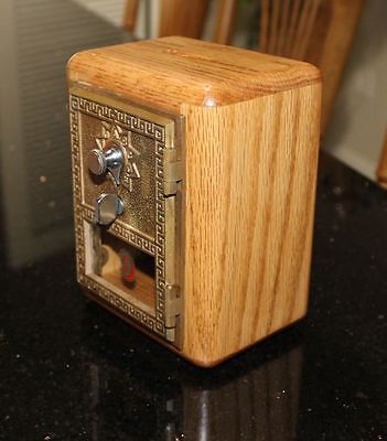
Let’s visualize a matching image pair.

pil_img = Image(filename=train_data[image_col_1][5])
display(pil_img)

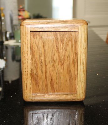
pil_img = Image(filename=train_data[image_col_2][5])
display(pil_img)

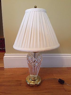
Here are two images that do not match.

pil_img = Image(filename=train_data[image_col_1][0])
display(pil_img)

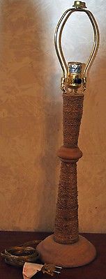
pil_img = Image(filename=train_data[image_col_2][0])
display(pil_img)

Train your Model

Ideally, we want to obtain a model that can return high/low scores for positive/negative image pairs. With AutoMM, we can easily train a model that captures the semantic relationship between images. Basically, it uses Swin Transformer to project each image into a high-dimensional vector and compute the cosine similarity of feature vectors.

With AutoMM, you just need to specify the query, response, and label column names and fit the model on the training dataset without worrying the implementation details.

from autogluon.multimodal import MultiModalPredictor
predictor = MultiModalPredictor(
        problem_type="image_similarity",
        query=image_col_1, # the column name of the first image
        response=image_col_2, # the column name of the second image
        label=label_col, # the label column name
        match_label=match_label, # the label indicating that query and response have the same semantic meanings.
        eval_metric='auc', # the evaluation metric
    )
    
# Fit the model
predictor.fit(
    train_data=train_data,
    time_limit=180,
)

Downloading: "https://github.com/SwinTransformer/storage/releases/download/v1.0.0/swin_base_patch4_window7_224_22kto1k.pth" to /home/ci/.cache/torch/hub/checkpoints/swin_base_patch4_window7_224_22kto1k.pth
No path specified. Models will be saved in: "AutogluonModels/ag-20230302_162103/"

<autogluon.multimodal.predictor.MultiModalPredictor at 0x7f5497a2bc70>

Evaluate on Test Dataset

You can evaluate the predictor on the test dataset to see how it performs with the roc_auc score:

score = predictor.evaluate(test_data)
print("evaluation score: ", score)

evaluation score:  {'roc_auc': 0.9480942628712825}

Predict on Image Pairs

Given new image pairs, we can predict whether they match or not.

pred = predictor.predict(test_data.head(3))
print(pred)

0    1
1    1
2    1
Name: Label, dtype: int64

The predictions use a naive probability threshold 0.5. That is, we choose the label with the probability larger than 0.5.

Predict Matching Probabilities

However, you can do more customized thresholding by getting probabilities.

proba = predictor.predict_proba(test_data.head(3))
print(proba)

          0         1
0  0.372953  0.627047
1  0.037047  0.962953
2  0.090726  0.909274

Extract Embeddings

You can also extract embeddings for each image of a pair.

embeddings_1 = predictor.extract_embedding({image_col_1: test_data[image_col_1][:5].tolist()})
print(embeddings_1.shape)
embeddings_2 = predictor.extract_embedding({image_col_2: test_data[image_col_2][:5].tolist()})
print(embeddings_2.shape)

(5, 1024)
(5, 1024)

Other Examples

You may go to AutoMM Examples to explore other examples about AutoMM.

Customization

To learn how to customize AutoMM, please refer to Customize AutoMM.