Automated Target Variable Analysis

In this section we explore automated dataset overview functionality.

Automated target variable analysis aims to automatically analyze and summarize the variable we are trying to predict ( label). The goal of this analysis is to take a deeper look into target variable structure and its relationship with other important variables in the dataset.

To simplify outliers and useful patterns discovery. This functionality introduces components which allow generating descriptive statistics and visualizing the target distribution and relationships between the target variable and other variables in the dataset.

Classification Example

We will start with getting titanic dataset and performing a quick one-line overview to get the information.

import pandas as pd

df_train = pd.read_csv('https://autogluon.s3.amazonaws.com/datasets/titanic/train.csv')
df_test = pd.read_csv('https://autogluon.s3.amazonaws.com/datasets/titanic/test.csv')
target_col = 'Survived'

The report consists of multiple parts: statistical information overview enriched with feature types detection and missing value counts focused only on the target variable.

Label Insights will highlight dataset features which require attention (i.e. class imbalance or out-of-domain data in test dataset).

The next component is feature distribution visualization. This is helpful for choosing data transformations and/or model selection. For regression tasks, the framework automatically fits multiple distributions available in scipy. The distributions with the best fit will be displayed on the chart. Distributions information will be displayed below the chart.

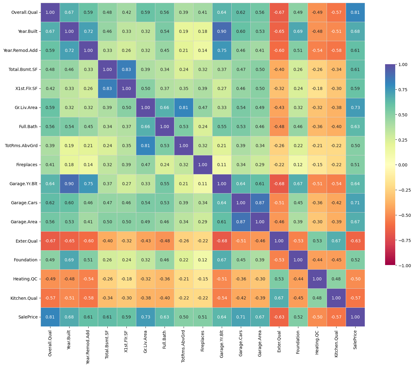
Next, the report will provide correlation analysis focusing only on highly-correlated features and visualization of their relationships with the target.

The last chart is a feature distance. It measures the similarity between features in a dataset. For example, if two variables are almost identical, their feature distance will be small. Understanding feature distance is useful in feature selection, where it can be used to identify which variables are redundant and should be considered for removal. To perform the analysis, we need just one line:

import autogluon.eda.auto as auto

auto.target_analysis(train_data=df_train, label=target_col)

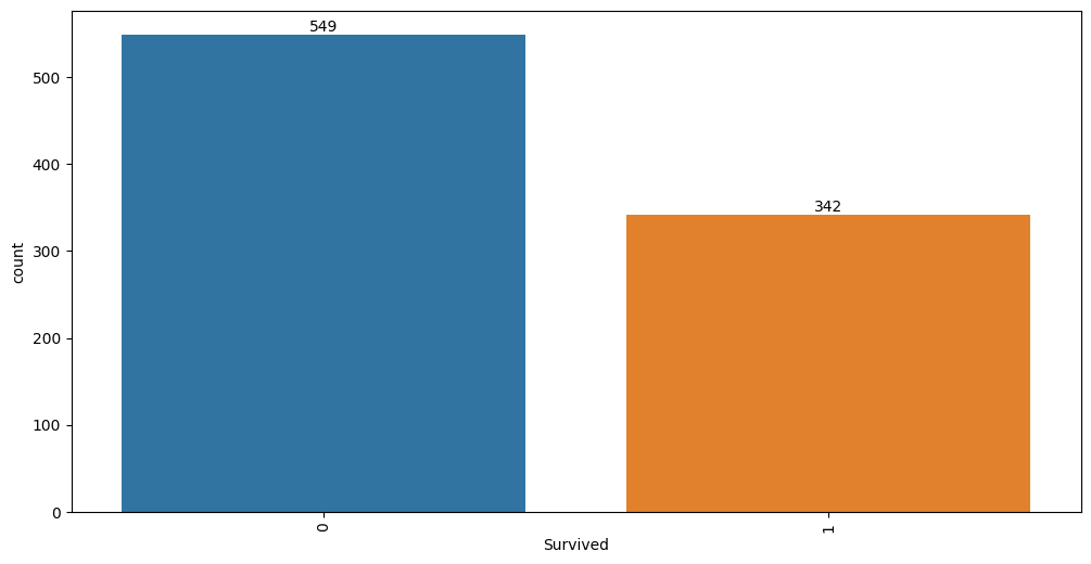
Target variable analysis

	count	mean	std	min	25%	50%	75%	max	dtypes	unique	missing_count	missing_ratio	raw_type	special_types
Survived	891	0.383838	0.486592	0.0	0.0	0.0	1.0	1.0	int64	2			int

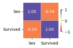
Target variable correlations

``train_data`` - ``spearman`` correlation matrix; focus: absolute correlation for ``Survived`` >= ``0.5``

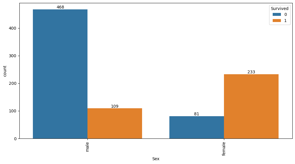
Feature interaction between ``Sex``/``Survived`` in ``train_data``

Regression Example

In the previous section we tried a classification example. Let’s try a regression. It has a few differences.

df_train = pd.read_csv('https://autogluon.s3.amazonaws.com/datasets/AmesHousingPriceRegression/train_data.csv')
df_test = pd.read_csv('https://autogluon.s3.amazonaws.com/datasets/AmesHousingPriceRegression/test_data.csv')
target_col = 'SalePrice'

auto.target_analysis(
    train_data=df_train, label=target_col,
    # Optional; default will try to fit all available distributions
    fit_distributions=['laplace_asymmetric', 'johnsonsu', 'exponnorm']
)

Target variable analysis

	count	mean	std	min	25%	50%	75%	max	dtypes	unique	missing_count	missing_ratio	raw_type	special_types
SalePrice	2344	181794.673635	82035.556894	12789.0	129000.0	160500.0	214000.0	755000.0	int64	918			int

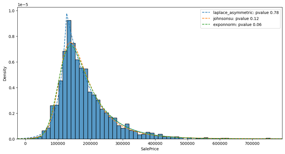
Distribution fits for target variable

• laplace_asymmetric

  • p-value: 0.784

  • Parameters: (kappa: 0.5531863345530886, loc: 127499.99999894513, scale: 43285.69671350392)

• johnsonsu

  • p-value: 0.120

  • Parameters: (a: -1.4433009164353976, b: 1.3922853595685476, loc: 97854.76437964055, scale: 52770.348354810485)

• exponnorm

  • p-value: 0.063

  • Parameters: (K: 2.62854289075631, loc: 107181.37845979724, scale: 28385.801254782047)

Target variable correlations

``train_data`` - ``spearman`` correlation matrix; focus: absolute correlation for ``SalePrice`` >= ``0.5``

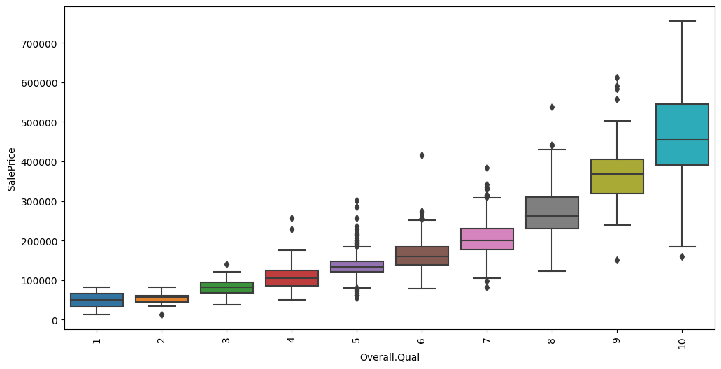
Feature interaction between ``Overall.Qual``/``SalePrice`` in ``train_data``

Feature interaction between ``Gr.Liv.Area``/``SalePrice`` in ``train_data``

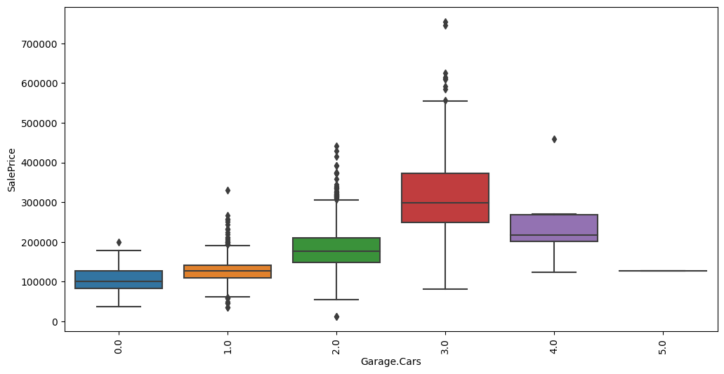
Feature interaction between ``Garage.Cars``/``SalePrice`` in ``train_data``

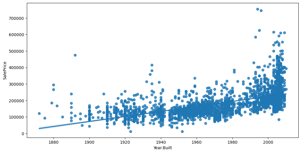
Feature interaction between ``Year.Built``/``SalePrice`` in ``train_data``

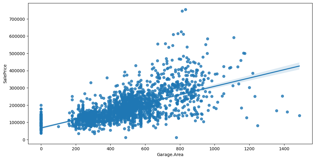
Feature interaction between ``Garage.Area``/``SalePrice`` in ``train_data``

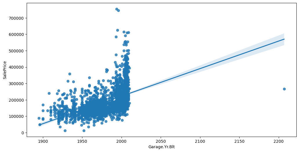
Feature interaction between ``Garage.Yr.Blt``/``SalePrice`` in ``train_data``

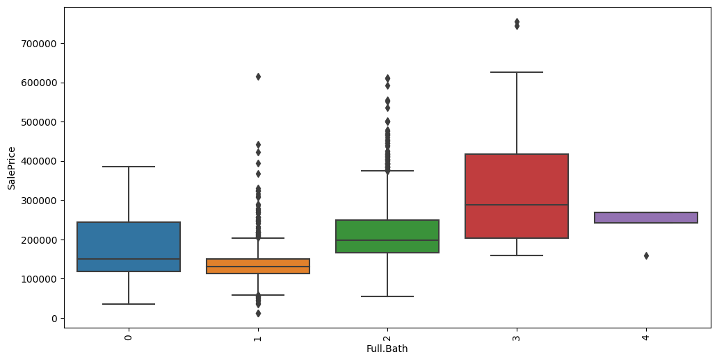
Feature interaction between ``Full.Bath``/``SalePrice`` in ``train_data``

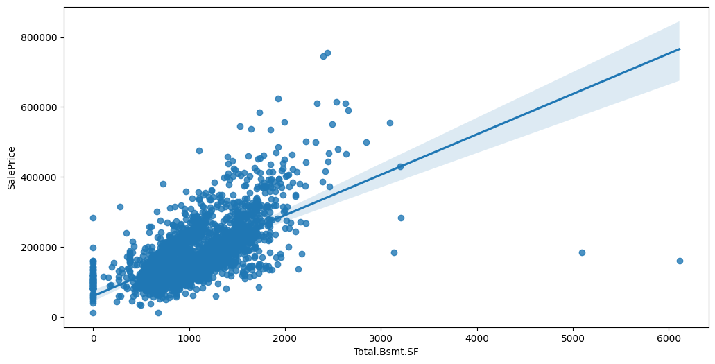
Feature interaction between ``Total.Bsmt.SF``/``SalePrice`` in ``train_data``

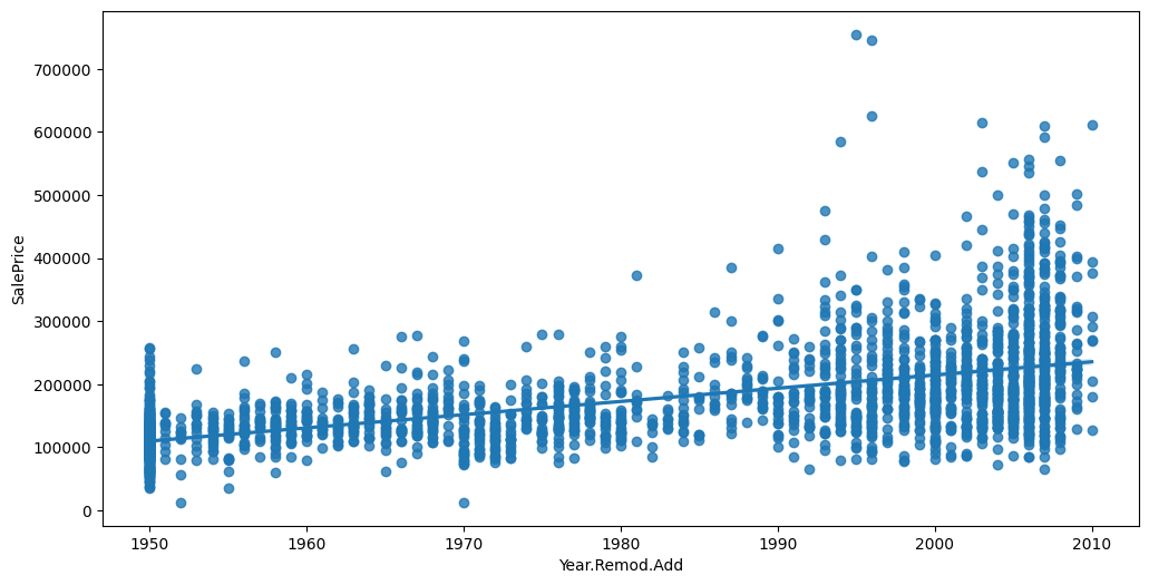
Feature interaction between ``Year.Remod.Add``/``SalePrice`` in ``train_data``

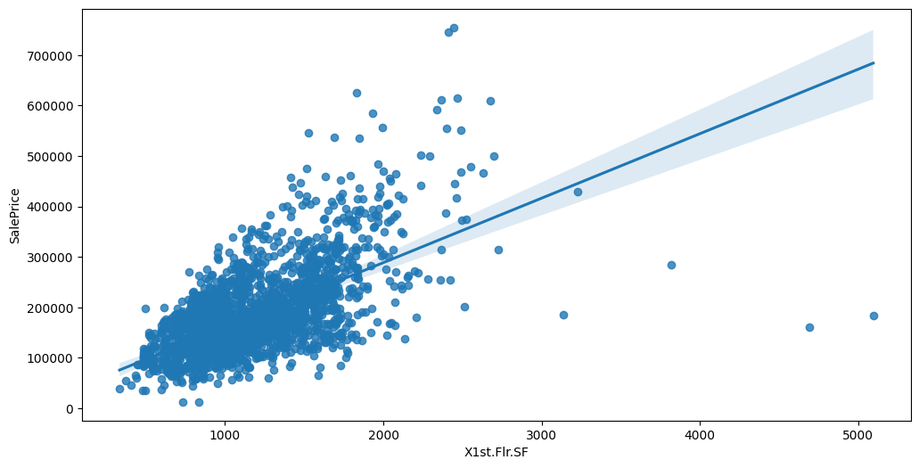
Feature interaction between ``X1st.Flr.SF``/``SalePrice`` in ``train_data``

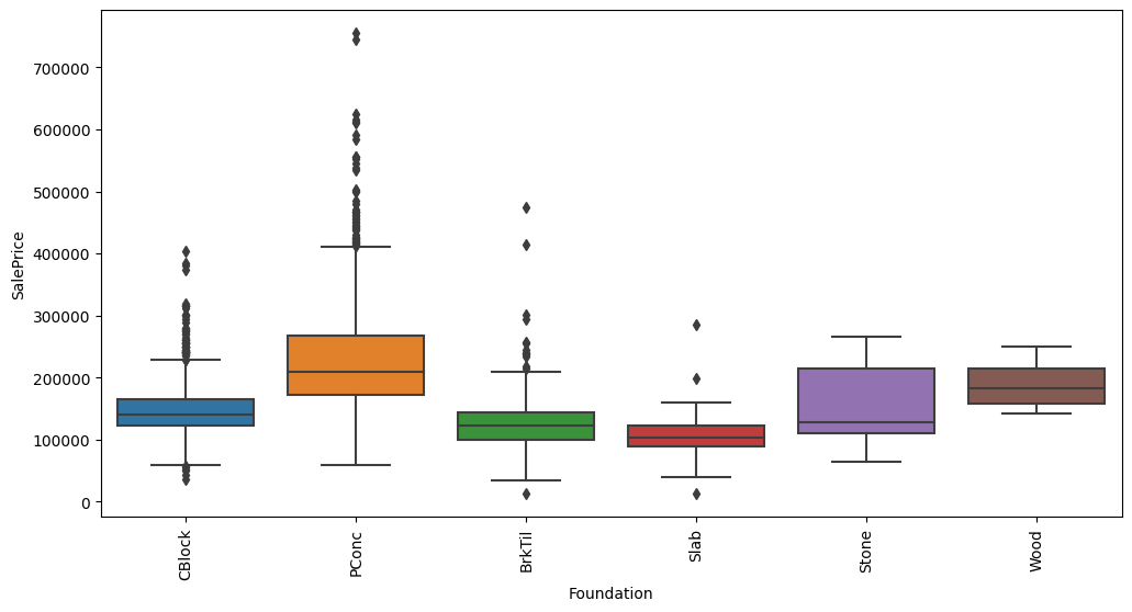
Feature interaction between ``Foundation``/``SalePrice`` in ``train_data``

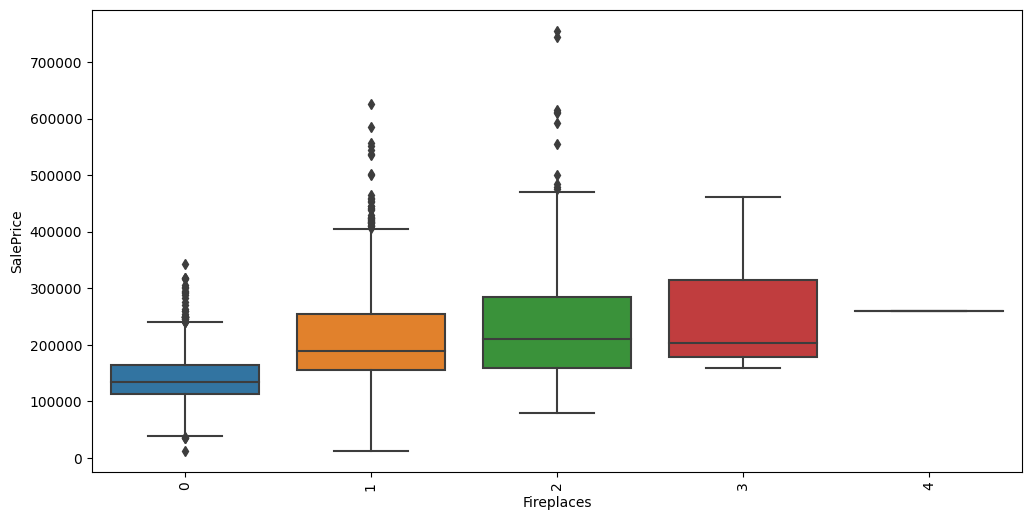
Feature interaction between ``Fireplaces``/``SalePrice`` in ``train_data``

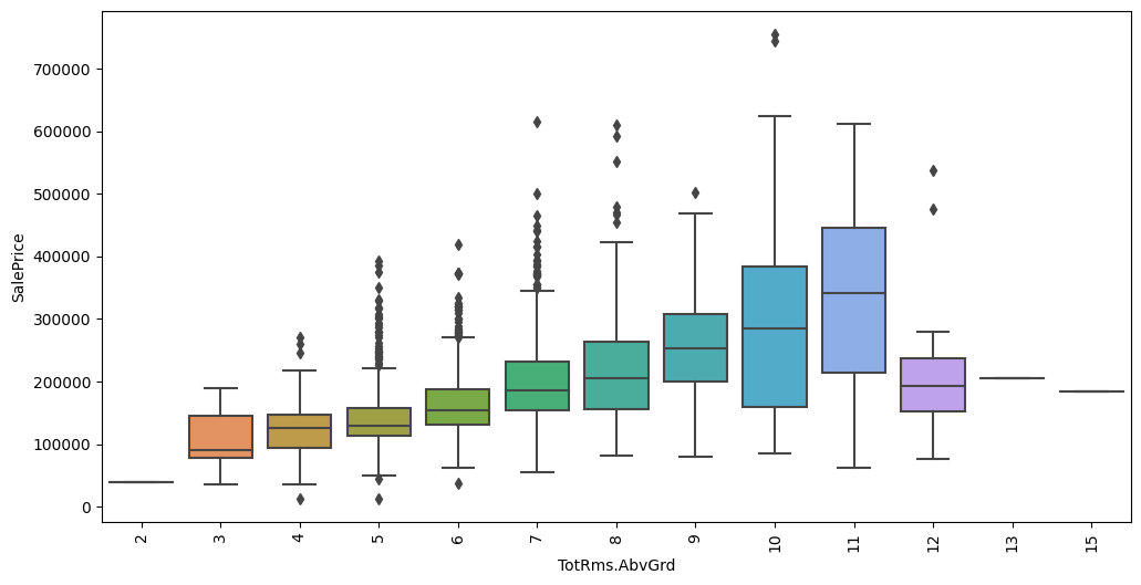
Feature interaction between ``TotRms.AbvGrd``/``SalePrice`` in ``train_data``

Feature interaction between ``Heating.QC``/``SalePrice`` in ``train_data``

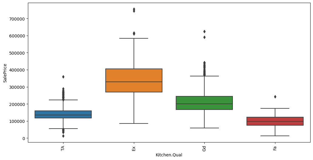
Feature interaction between ``Kitchen.Qual``/``SalePrice`` in ``train_data``

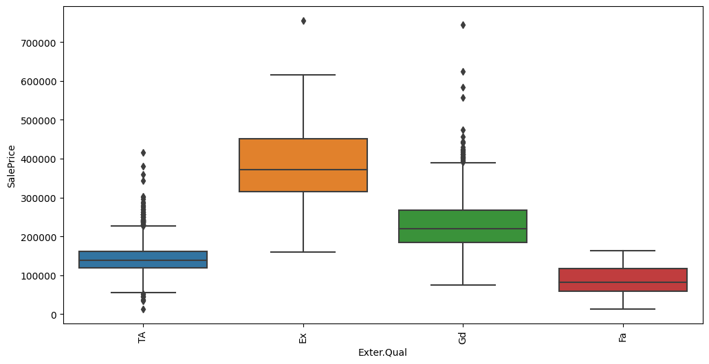
Feature interaction between ``Exter.Qual``/``SalePrice`` in ``train_data``