
Text Prediction - Quick Start
Here we briefly demonstrate the TextPredictor, which helps you
automatically train and deploy models for various Natural Language
Processing (NLP) tasks. This tutorial presents two examples of NLP
tasks:
The general usage of the TextPredictor is similar to AutoGluon’s
TabularPredictor. We format NLP datasets as tables where certain
columns contain text fields and a special column contains the labels to
predict, and each row corresponds to one training example. Here, the
labels can be discrete categories (classification) or numerical values
(regression).
%matplotlib inline

import numpy as np
import warnings
import matplotlib.pyplot as plt
warnings.filterwarnings('ignore')
np.random.seed(123)
Sentiment Analysis Task
First, we consider the Stanford Sentiment Treebank (SST) dataset, which consists of movie reviews and their associated sentiment. Given a new movie review, the goal is to predict the sentiment reflected in the text (in this case a binary classification, where reviews are labeled as 1 if they convey a positive opinion and labeled as 0 otherwise). Let’s first load and look at the data, noting the labels are stored in a column called label.
from autogluon.core.utils.loaders.load_pd import load
train_data = load('https://autogluon-text.s3-accelerate.amazonaws.com/glue/sst/train.parquet')
test_data = load('https://autogluon-text.s3-accelerate.amazonaws.com/glue/sst/dev.parquet')
subsample_size = 1000  # subsample data for faster demo, try setting this to larger values
train_data = train_data.sample(n=subsample_size, random_state=0)
train_data.head(10)
| sentence | label | |
|---|---|---|
| 43787 | very pleasing at its best moments | 1 |
| 16159 | , american chai is enough to make you put away... | 0 |
| 59015 | too much like an infomercial for ram dass 's l... | 0 |
| 5108 | a stirring visual sequence | 1 |
| 67052 | cool visual backmasking | 1 |
| 35938 | hard ground | 0 |
| 49879 | the striking , quietly vulnerable personality ... | 1 |
| 51591 | pan nalin 's exposition is beautiful and myste... | 1 |
| 56780 | wonderfully loopy | 1 |
| 28518 | most beautiful , evocative | 1 |
Above the data happen to be stored in a
Parquet table
format, but you can also directly load() data from a
CSV file
instead. While here we load files from AWS S3 cloud
storage,
these could instead be local files on your machine. After loading,
train_data is simply a Pandas
DataFrame,
where each row represents a different training example (for machine
learning to be appropriate, the rows should be independent and
identically distributed).
Training
To ensure this tutorial runs quickly, we simply call fit() with a
subset of 1000 training examples and limit its runtime to approximately
1 minute. To achieve reasonable performance in your applications, you
are recommended to set much longer time_limit (eg. 1 hour), or do
not specify time_limit at all (time_limit=None).
from autogluon.text import TextPredictor

predictor = TextPredictor(label='label', eval_metric='acc', path='./ag_sst')
predictor.fit(train_data, time_limit=60)
Problem Type="binary"
Column Types:
   - "sentence": text
   - "label": categorical

NumPy-shape semantics has been activated in your code. This is required for creating and manipulating scalar and zero-size tensors, which were not supported in MXNet before, as in the official NumPy library. Please DO NOT manually deactivate this semantics while using mxnet.numpy and mxnet.numpy_extension modules.
The GluonNLP V0 backend is used. We will use 8 cpus and 1 gpus to train each trial.
All Logs will be saved to /var/lib/jenkins/workspace/workspace/autogluon-tutorial-text-v3/docs/_build/eval/tutorials/text_prediction/ag_sst/task0/training.log
Fitting and transforming the train data...
Done! Preprocessor saved to /var/lib/jenkins/workspace/workspace/autogluon-tutorial-text-v3/docs/_build/eval/tutorials/text_prediction/ag_sst/task0/preprocessor.pkl
Process dev set...
Done!
Max length for chunking text: 64, Stochastic chunk: Train-False/Test-False, Test #repeat: 1.
#Total Params/Fixed Params=108990466/0
Using gradient accumulation. Global batch size = 128
Local training results will be saved to /var/lib/jenkins/workspace/workspace/autogluon-tutorial-text-v3/docs/_build/eval/tutorials/text_prediction/ag_sst/task0/results_local.jsonl.
[Iter 1/70, Epoch 0] train loss=8.76e-01, gnorm=9.82e+00, lr=1.43e-05, #samples processed=128, #sample per second=86.06. ETA=1.71min
[Iter 2/70, Epoch 0] train loss=7.94e-01, gnorm=6.16e+00, lr=2.86e-05, #samples processed=128, #sample per second=150.43. ETA=1.33min
[Iter 2/70, Epoch 0] valid f1=7.2204e-01, mcc=0.0000e+00, roc_auc=4.2305e-01, accuracy=5.6500e-01, log_loss=1.0976e+00, time spent=0.460s, total time spent=0.07min. Find new best=True, Find new top-3=True
[Iter 3/70, Epoch 0] train loss=1.29e+00, gnorm=1.51e+01, lr=4.29e-05, #samples processed=128, #sample per second=52.81. ETA=1.77min
[Iter 4/70, Epoch 0] train loss=1.15e+00, gnorm=1.27e+01, lr=5.71e-05, #samples processed=128, #sample per second=160.16. ETA=1.53min
[Iter 4/70, Epoch 0] valid f1=5.6716e-01, mcc=1.4791e-01, roc_auc=6.2750e-01, accuracy=5.6500e-01, log_loss=6.9451e-01, time spent=0.447s, total time spent=0.12min. Find new best=True, Find new top-3=True
[Iter 5/70, Epoch 0] train loss=6.92e-01, gnorm=6.95e+00, lr=7.14e-05, #samples processed=128, #sample per second=49.15. ETA=1.77min
[Iter 6/70, Epoch 0] train loss=6.23e-01, gnorm=1.95e+01, lr=8.57e-05, #samples processed=128, #sample per second=150.99. ETA=1.60min
[Iter 6/70, Epoch 0] valid f1=7.1947e-01, mcc=7.6355e-02, roc_auc=7.2882e-01, accuracy=5.7500e-01, log_loss=6.7021e-01, time spent=0.448s, total time spent=0.19min. Find new best=True, Find new top-3=True
[Iter 7/70, Epoch 0] train loss=6.59e-01, gnorm=7.78e+00, lr=1.00e-04, #samples processed=128, #sample per second=43.79. ETA=1.79min
[Iter 8/70, Epoch 1] train loss=7.61e-01, gnorm=1.45e+01, lr=9.84e-05, #samples processed=128, #sample per second=163.67. ETA=1.64min
[Iter 8/70, Epoch 1] valid f1=5.5866e-01, mcc=2.7262e-01, roc_auc=6.9301e-01, accuracy=6.0500e-01, log_loss=6.6740e-01, time spent=0.453s, total time spent=0.25min. Find new best=True, Find new top-3=True
[Iter 9/70, Epoch 1] train loss=7.56e-01, gnorm=5.62e+00, lr=9.68e-05, #samples processed=128, #sample per second=39.48. ETA=1.80min
[Iter 10/70, Epoch 1] train loss=7.24e-01, gnorm=5.96e+00, lr=9.52e-05, #samples processed=128, #sample per second=158.05. ETA=1.68min
[Iter 10/70, Epoch 1] valid f1=7.5839e-01, mcc=3.2452e-01, roc_auc=8.7845e-01, accuracy=6.4000e-01, log_loss=5.7693e-01, time spent=0.451s, total time spent=0.32min. Find new best=True, Find new top-3=True
[Iter 11/70, Epoch 1] train loss=6.31e-01, gnorm=4.66e+00, lr=9.37e-05, #samples processed=128, #sample per second=39.35. ETA=1.79min
[Iter 12/70, Epoch 1] train loss=5.70e-01, gnorm=5.85e+00, lr=9.21e-05, #samples processed=128, #sample per second=162.56. ETA=1.68min
[Iter 12/70, Epoch 1] valid f1=7.9397e-01, mcc=6.1951e-01, roc_auc=9.1527e-01, accuracy=7.9500e-01, log_loss=4.7745e-01, time spent=0.459s, total time spent=0.39min. Find new best=True, Find new top-3=True
[Iter 13/70, Epoch 1] train loss=5.57e-01, gnorm=5.38e+00, lr=9.05e-05, #samples processed=128, #sample per second=40.44. ETA=1.75min
[Iter 14/70, Epoch 1] train loss=3.91e-01, gnorm=3.17e+00, lr=8.89e-05, #samples processed=128, #sample per second=165.05. ETA=1.65min
[Iter 14/70, Epoch 1] valid f1=8.6381e-01, mcc=6.6579e-01, roc_auc=9.0927e-01, accuracy=8.2500e-01, log_loss=4.5740e-01, time spent=0.457s, total time spent=0.46min. Find new best=True, Find new top-3=True
[Iter 15/70, Epoch 2] train loss=3.69e-01, gnorm=6.26e+00, lr=8.73e-05, #samples processed=128, #sample per second=37.78. ETA=1.72min
[Iter 16/70, Epoch 2] train loss=2.38e-01, gnorm=2.43e+00, lr=8.57e-05, #samples processed=128, #sample per second=165.79. ETA=1.63min
[Iter 16/70, Epoch 2] valid f1=9.0909e-01, mcc=7.9963e-01, roc_auc=9.5209e-01, accuracy=9.0000e-01, log_loss=3.1594e-01, time spent=0.457s, total time spent=0.52min. Find new best=True, Find new top-3=True
[Iter 17/70, Epoch 2] train loss=3.59e-01, gnorm=5.29e+00, lr=8.41e-05, #samples processed=128, #sample per second=39.19. ETA=1.67min
[Iter 18/70, Epoch 2] train loss=2.87e-01, gnorm=5.75e+00, lr=8.25e-05, #samples processed=128, #sample per second=160.78. ETA=1.59min
[Iter 18/70, Epoch 2] valid f1=8.8000e-01, mcc=7.0770e-01, roc_auc=9.4660e-01, accuracy=8.5000e-01, log_loss=4.6460e-01, time spent=0.462s, total time spent=0.57min. Find new best=False, Find new top-3=True
[Iter 19/70, Epoch 2] train loss=3.11e-01, gnorm=8.02e+00, lr=8.10e-05, #samples processed=128, #sample per second=56.57. ETA=1.58min
[Iter 20/70, Epoch 2] train loss=1.73e-01, gnorm=2.98e+00, lr=7.94e-05, #samples processed=128, #sample per second=169.35. ETA=1.50min
[Iter 20/70, Epoch 2] valid f1=8.8393e-01, mcc=7.3638e-01, roc_auc=9.4395e-01, accuracy=8.7000e-01, log_loss=3.2271e-01, time spent=0.458s, total time spent=0.62min. Find new best=False, Find new top-3=True
[Iter 21/70, Epoch 2] train loss=3.55e-01, gnorm=4.42e+00, lr=7.78e-05, #samples processed=128, #sample per second=57.90. ETA=1.49min
[Iter 22/70, Epoch 3] train loss=2.36e-01, gnorm=8.88e+00, lr=7.62e-05, #samples processed=128, #sample per second=153.43. ETA=1.42min
[Iter 22/70, Epoch 3] valid f1=8.7336e-01, mcc=7.0417e-01, roc_auc=9.4233e-01, accuracy=8.5500e-01, log_loss=3.1476e-01, time spent=0.457s, total time spent=0.67min. Find new best=False, Find new top-3=True
[Iter 23/70, Epoch 3] train loss=1.99e-01, gnorm=6.51e+00, lr=7.46e-05, #samples processed=128, #sample per second=58.19. ETA=1.41min
[Iter 24/70, Epoch 3] train loss=3.36e-01, gnorm=8.62e+00, lr=7.30e-05, #samples processed=128, #sample per second=167.11. ETA=1.34min
[Iter 24/70, Epoch 3] valid f1=8.6957e-01, mcc=6.8006e-01, roc_auc=9.3999e-01, accuracy=8.3500e-01, log_loss=4.5034e-01, time spent=0.457s, total time spent=0.71min. Find new best=False, Find new top-3=False
[Iter 25/70, Epoch 3] train loss=2.44e-01, gnorm=4.81e+00, lr=7.14e-05, #samples processed=128, #sample per second=101.26. ETA=1.30min
[Iter 26/70, Epoch 3] train loss=1.69e-01, gnorm=1.84e+00, lr=6.98e-05, #samples processed=128, #sample per second=172.41. ETA=1.24min
[Iter 26/70, Epoch 3] valid f1=8.9498e-01, mcc=7.7011e-01, roc_auc=9.4426e-01, accuracy=8.8500e-01, log_loss=3.3178e-01, time spent=0.453s, total time spent=0.76min. Find new best=False, Find new top-3=True
[Iter 27/70, Epoch 3] train loss=2.08e-01, gnorm=2.65e+00, lr=6.83e-05, #samples processed=128, #sample per second=53.41. ETA=1.23min
[Iter 28/70, Epoch 3] train loss=1.86e-01, gnorm=4.24e+00, lr=6.67e-05, #samples processed=128, #sample per second=166.20. ETA=1.18min
[Iter 28/70, Epoch 3] valid f1=8.8136e-01, mcc=7.1518e-01, roc_auc=9.3317e-01, accuracy=8.6000e-01, log_loss=3.9546e-01, time spent=0.453s, total time spent=0.79min. Find new best=False, Find new top-3=False
[Iter 29/70, Epoch 4] train loss=9.32e-02, gnorm=2.09e+00, lr=6.51e-05, #samples processed=128, #sample per second=102.40. ETA=1.14min
[Iter 30/70, Epoch 4] train loss=2.13e-01, gnorm=7.57e+00, lr=6.35e-05, #samples processed=128, #sample per second=162.25. ETA=1.09min
[Iter 30/70, Epoch 4] valid f1=8.5490e-01, mcc=6.3946e-01, roc_auc=9.2290e-01, accuracy=8.1500e-01, log_loss=6.5264e-01, time spent=0.464s, total time spent=0.83min. Find new best=False, Find new top-3=False
[Iter 31/70, Epoch 4] train loss=1.75e-01, gnorm=6.40e+00, lr=6.19e-05, #samples processed=128, #sample per second=100.83. ETA=1.06min
[Iter 32/70, Epoch 4] train loss=2.13e-01, gnorm=7.47e+00, lr=6.03e-05, #samples processed=128, #sample per second=158.83. ETA=1.02min
[Iter 32/70, Epoch 4] valid f1=8.8333e-01, mcc=7.1741e-01, roc_auc=9.4039e-01, accuracy=8.6000e-01, log_loss=4.1703e-01, time spent=0.463s, total time spent=0.86min. Find new best=False, Find new top-3=False
Training completed. Auto-saving to "./ag_sst/". For loading the model, you can use predictor = TextPredictor.load("./ag_sst/")
<autogluon.text.text_prediction.predictor.predictor.TextPredictor at 0x7f4dd5192750>
Above we specify that: the column named label contains the label values to predict, AutoGluon should optimize its predictions for the accuracy evaluation metric, trained models should be saved in the ag_sst folder, and training should run for around 60 seconds.
Evaluation
After training, we can easily evaluate our predictor on separate test data formatted similarly to our training data.
test_score = predictor.evaluate(test_data)
print('Accuracy = {:.2f}%'.format(test_score * 100))
Accuracy = 89.33%
By default, evaluate() will report the evaluation metric previously
specified, which is accuracy in our example. You may also specify
additional metrics, e.g. F1 score, when calling evaluate.
test_score = predictor.evaluate(test_data, metrics=['acc', 'f1'])
print(test_score)
{'acc': 0.893348623853211, 'f1': 0.890716803760282}
Prediction
And you can easily obtain predictions from these models by calling
predictor.predict().
sentence1 = "it's a charming and often affecting journey."
sentence2 = "It's slow, very, very, very slow."
predictions = predictor.predict({'sentence': [sentence1, sentence2]})
print('"Sentence":', sentence1, '"Predicted Sentiment":', predictions[0])
print('"Sentence":', sentence2, '"Predicted Sentiment":', predictions[1])
"Sentence": it's a charming and often affecting journey. "Predicted Sentiment": 1
"Sentence": It's slow, very, very, very slow. "Predicted Sentiment": 0
For classification tasks, you can ask for predicted class-probabilities instead of predicted classes.
probs = predictor.predict_proba({'sentence': [sentence1, sentence2]})
print('"Sentence":', sentence1, '"Predicted Class-Probabilities":', probs[0])
print('"Sentence":', sentence2, '"Predicted Class-Probabilities":', probs[1])
"Sentence": it's a charming and often affecting journey. "Predicted Class-Probabilities": 0    0.002646
1    0.974943
Name: 0, dtype: float32
"Sentence": It's slow, very, very, very slow. "Predicted Class-Probabilities": 0    0.997355
1    0.025057
Name: 1, dtype: float32
We can just as easily produce predictions over an entire dataset.
test_predictions = predictor.predict(test_data)
test_predictions.head()
0    1
1    0
2    1
3    1
4    0
Name: label, dtype: int64
Intermediate Training Results
After training, you can explore intermediate training results in
predictor.results.
predictor.results.tail(3)
| iteration | report_idx | epoch | f1 | mcc | roc_auc | accuracy | log_loss | find_better | find_new_topn | nbest_stat | elapsed_time | reward_attr | eval_metric | exp_dir | |
|---|---|---|---|---|---|---|---|---|---|---|---|---|---|---|---|
| 14 | 30 | 15 | 4 | 0.854902 | 0.639459 | 0.922897 | 0.815 | 0.652641 | False | False | [[0.87, 0.9, 0.885], [20, 16, 26]] | 49 | 0.815 | accuracy | /var/lib/jenkins/workspace/workspace/autogluon... |
| 15 | 32 | 16 | 4 | 0.883333 | 0.717406 | 0.940393 | 0.860 | 0.417029 | False | False | [[0.87, 0.9, 0.885], [20, 16, 26]] | 51 | 0.860 | accuracy | /var/lib/jenkins/workspace/workspace/autogluon... |
| 16 | 16 | 17 | 2 | 0.909091 | 0.799631 | 0.952090 | 0.900 | 0.315937 | True | True | [[0.825, 0.9, 0.795], [14, 16, 12]] | 31 | 0.900 | accuracy | /var/lib/jenkins/workspace/workspace/autogluon... |
Save and Load
The trained predictor is automatically saved at the end of fit(),
and you can easily reload it.
loaded_predictor = TextPredictor.load('ag_sst')
loaded_predictor.predict_proba({'sentence': [sentence1, sentence2]})
| 0 | 1 | |
|---|---|---|
| 0 | 0.002646 | 0.997355 |
| 1 | 0.974943 | 0.025057 |
You can also save the predictor to any location by calling .save().
loaded_predictor.save('my_saved_dir')
loaded_predictor2 = TextPredictor.load('my_saved_dir')
loaded_predictor2.predict_proba({'sentence': [sentence1, sentence2]})
| 0 | 1 | |
|---|---|---|
| 0 | 0.002646 | 0.997355 |
| 1 | 0.974943 | 0.025057 |
Extract Embeddings
You can also use a trained predictor to extract embeddings that maps each row of the data table to an embedding vector extracted from intermediate neural network representations of the row.
embeddings = predictor.extract_embedding(test_data)
print(embeddings)
[[-1.0801306  -0.44154665 -1.0147676  ... -0.8042417   0.5623589
   0.51314175]
 [-0.5288651   0.13702041 -0.45935678 ...  0.17704543  0.35587373
  -0.13050948]
 [-0.7904423  -0.1516396  -0.736847   ... -0.57204205  0.5236889
   0.3740344 ]
 ...
 [-0.4152624   0.20381683 -0.39514995 ... -0.22893398  0.23090875
   0.36273792]
 [-0.39312404  0.30050468 -0.6993964  ...  0.1369121   0.16843818
   0.09883293]
 [-0.89676505  0.12524071 -0.3635128  ... -0.51871604 -0.04470562
   0.11770649]]
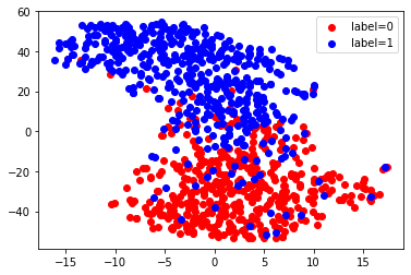
Here, we use TSNE to visualize these extracted embeddings. We can see that there are two clusters corresponding to our two labels, since this network has been trained to discriminate between these labels.
from sklearn.manifold import TSNE
X_embedded = TSNE(n_components=2, random_state=123).fit_transform(embeddings)
for val, color in [(0, 'red'), (1, 'blue')]:
    idx = (test_data['label'].to_numpy() == val).nonzero()
    plt.scatter(X_embedded[idx, 0], X_embedded[idx, 1], c=color, label=f'label={val}')
plt.legend(loc='best')
<matplotlib.legend.Legend at 0x7f4d1d7fe8d0>
Sentence Similarity Task
Next, let’s use AutoGluon to train a model for evaluating how semantically similar two sentences are. We use the Semantic Textual Similarity Benchmark dataset for illustration.
sts_train_data = load('https://autogluon-text.s3-accelerate.amazonaws.com/glue/sts/train.parquet')[['sentence1', 'sentence2', 'score']]
sts_test_data = load('https://autogluon-text.s3-accelerate.amazonaws.com/glue/sts/dev.parquet')[['sentence1', 'sentence2', 'score']]
sts_train_data.head(10)
Loaded data from: https://autogluon-text.s3-accelerate.amazonaws.com/glue/sts/train.parquet | Columns = 4 / 4 | Rows = 5749 -> 5749
Loaded data from: https://autogluon-text.s3-accelerate.amazonaws.com/glue/sts/dev.parquet | Columns = 4 / 4 | Rows = 1500 -> 1500
| sentence1 | sentence2 | score | |
|---|---|---|---|
| 0 | A plane is taking off. | An air plane is taking off. | 5.00 |
| 1 | A man is playing a large flute. | A man is playing a flute. | 3.80 |
| 2 | A man is spreading shreded cheese on a pizza. | A man is spreading shredded cheese on an uncoo... | 3.80 |
| 3 | Three men are playing chess. | Two men are playing chess. | 2.60 |
| 4 | A man is playing the cello. | A man seated is playing the cello. | 4.25 |
| 5 | Some men are fighting. | Two men are fighting. | 4.25 |
| 6 | A man is smoking. | A man is skating. | 0.50 |
| 7 | The man is playing the piano. | The man is playing the guitar. | 1.60 |
| 8 | A man is playing on a guitar and singing. | A woman is playing an acoustic guitar and sing... | 2.20 |
| 9 | A person is throwing a cat on to the ceiling. | A person throws a cat on the ceiling. | 5.00 |
In this data, the column named score contains numerical values (which we’d like to predict) that are human-annotated similarity scores for each given pair of sentences.
print('Min score=', min(sts_train_data['score']), ', Max score=', max(sts_train_data['score']))
Min score= 0.0 , Max score= 5.0
Let’s train a regression model to predict these scores. Note that we
only need to specify the label column and AutoGluon automatically
determines the type of prediction problem and an appropriate loss
function. Once again, you should increase the short time_limit below
to obtain reasonable performance in your own applications.
predictor_sts = TextPredictor(label='score', path='./ag_sts')
predictor_sts.fit(sts_train_data, time_limit=60)
Problem Type="regression"
Column Types:
   - "sentence1": text
   - "sentence2": text
   - "score": numerical

The GluonNLP V0 backend is used. We will use 8 cpus and 1 gpus to train each trial.
All Logs will be saved to /var/lib/jenkins/workspace/workspace/autogluon-tutorial-text-v3/docs/_build/eval/tutorials/text_prediction/ag_sts/task0/training.log
Fitting and transforming the train data...
Done! Preprocessor saved to /var/lib/jenkins/workspace/workspace/autogluon-tutorial-text-v3/docs/_build/eval/tutorials/text_prediction/ag_sts/task0/preprocessor.pkl
Process dev set...
Done!
Max length for chunking text: 128, Stochastic chunk: Train-False/Test-False, Test #repeat: 1.
#Total Params/Fixed Params=108990337/0
Using gradient accumulation. Global batch size = 128
Local training results will be saved to /var/lib/jenkins/workspace/workspace/autogluon-tutorial-text-v3/docs/_build/eval/tutorials/text_prediction/ag_sts/task0/results_local.jsonl.
[Iter 3/410, Epoch 0] train loss=1.43e+00, gnorm=1.50e+01, lr=7.32e-06, #samples processed=384, #sample per second=95.68. ETA=9.06min
[Iter 6/410, Epoch 0] train loss=1.18e+00, gnorm=1.02e+01, lr=1.46e-05, #samples processed=384, #sample per second=110.54. ETA=8.40min
[Iter 9/410, Epoch 0] train loss=9.54e-01, gnorm=8.82e+00, lr=2.20e-05, #samples processed=384, #sample per second=94.49. ETA=8.58min
[Iter 9/410, Epoch 0] valid r2=3.1820e-01, root_mean_squared_error=1.2272e+00, mean_absolute_error=9.8191e-01, time spent=2.102s, total time spent=0.25min. Find new best=True, Find new top-3=True
[Iter 12/410, Epoch 0] train loss=7.15e-01, gnorm=5.53e+00, lr=2.93e-05, #samples processed=384, #sample per second=52.09. ETA=10.46min
[Iter 15/410, Epoch 0] train loss=6.22e-01, gnorm=1.11e+01, lr=3.66e-05, #samples processed=384, #sample per second=100.15. ETA=9.99min
[Iter 18/410, Epoch 0] train loss=5.01e-01, gnorm=1.36e+01, lr=4.39e-05, #samples processed=384, #sample per second=111.31. ETA=9.51min
[Iter 18/410, Epoch 0] valid r2=4.9846e-01, root_mean_squared_error=1.0525e+00, mean_absolute_error=8.4806e-01, time spent=2.101s, total time spent=0.50min. Find new best=True, Find new top-3=True
[Iter 21/410, Epoch 0] train loss=5.39e-01, gnorm=7.75e+00, lr=5.12e-05, #samples processed=384, #sample per second=49.05. ETA=10.51min
[Iter 24/410, Epoch 0] train loss=5.38e-01, gnorm=3.06e+00, lr=5.85e-05, #samples processed=384, #sample per second=103.70. ETA=10.12min
[Iter 27/410, Epoch 0] train loss=4.42e-01, gnorm=2.78e+00, lr=6.59e-05, #samples processed=384, #sample per second=93.21. ETA=9.90min
[Iter 27/410, Epoch 0] valid r2=6.8437e-01, root_mean_squared_error=8.3495e-01, mean_absolute_error=6.6289e-01, time spent=2.099s, total time spent=0.76min. Find new best=True, Find new top-3=True
[Iter 30/410, Epoch 0] train loss=3.40e-01, gnorm=6.81e+00, lr=7.32e-05, #samples processed=384, #sample per second=51.28. ETA=10.42min
[Iter 33/410, Epoch 0] train loss=4.79e-01, gnorm=8.57e+00, lr=8.05e-05, #samples processed=384, #sample per second=93.00. ETA=10.18min
[Iter 36/410, Epoch 0] train loss=3.50e-01, gnorm=8.05e+00, lr=8.78e-05, #samples processed=384, #sample per second=97.41. ETA=9.94min
[Iter 36/410, Epoch 0] valid r2=6.4901e-01, root_mean_squared_error=8.8048e-01, mean_absolute_error=7.1154e-01, time spent=2.097s, total time spent=1.01min. Find new best=False, Find new top-3=True
Training completed. Auto-saving to "./ag_sts/". For loading the model, you can use predictor = TextPredictor.load("./ag_sts/")
<autogluon.text.text_prediction.predictor.predictor.TextPredictor at 0x7f4d3403c650>
We again evaluate our trained model’s performance on separate test data. Below we choose to compute the following metrics: RMSE, Pearson Correlation, and Spearman Correlation.
test_score = predictor_sts.evaluate(sts_test_data, metrics=['rmse', 'pearsonr', 'spearmanr'])
print('RMSE = {:.2f}'.format(test_score['rmse']))
print('PEARSONR = {:.4f}'.format(test_score['pearsonr']))
print('SPEARMANR = {:.4f}'.format(test_score['spearmanr']))
RMSE = 0.73
PEARSONR = 0.8771
SPEARMANR = 0.8770
Let’s use our model to predict the similarity score between a few sentences.
sentences = ['The child is riding a horse.',
             'The young boy is riding a horse.',
             'The young man is riding a horse.',
             'The young man is riding a bicycle.']

score1 = predictor_sts.predict({'sentence1': [sentences[0]],
                                'sentence2': [sentences[1]]}, as_pandas=False)

score2 = predictor_sts.predict({'sentence1': [sentences[0]],
                                'sentence2': [sentences[2]]}, as_pandas=False)

score3 = predictor_sts.predict({'sentence1': [sentences[0]],
                                'sentence2': [sentences[3]]}, as_pandas=False)
print(score1, score2, score3)
[4.2363434] [2.9265797] [0.87026674]
Although the TextPredictor is only designed for classification and
regression tasks, it can directly be used for many NLP tasks if you
properly format them into a data table. Note that there can be many text
columns in this data table. Refer to the TextPredictor
documentation
to see all of the available methods/options.
Unlike TabularPredictor which trains/ensembles many different kinds
of models, TextPredictor fits only Transformer neural network
models. These are fit to your data via transfer learning from pretrained
NLP models like: BERT,
ALBERT, and
ELECTRA.
TextPredictor also enables training on multi-modal data tables that
contain text, numeric and categorical columns, and the neural network
hyperparameter can be automatically tuned with Hyperparameter
Optimization (HPO), which will be introduced in the other tutorials.
Note: TextPredictor depends on the
GluonNLP package. Due to an ongoing
upgrade of GluonNLP, we are currently using a custom version of the
package:
autogluon-contrib-nlp.
In a future release, AutoGluon will support the official GluonNLP 1.0,
but the APIs demonstrated here will remain the same.