Search Algorithms
AutoGluon System Implementation Logic
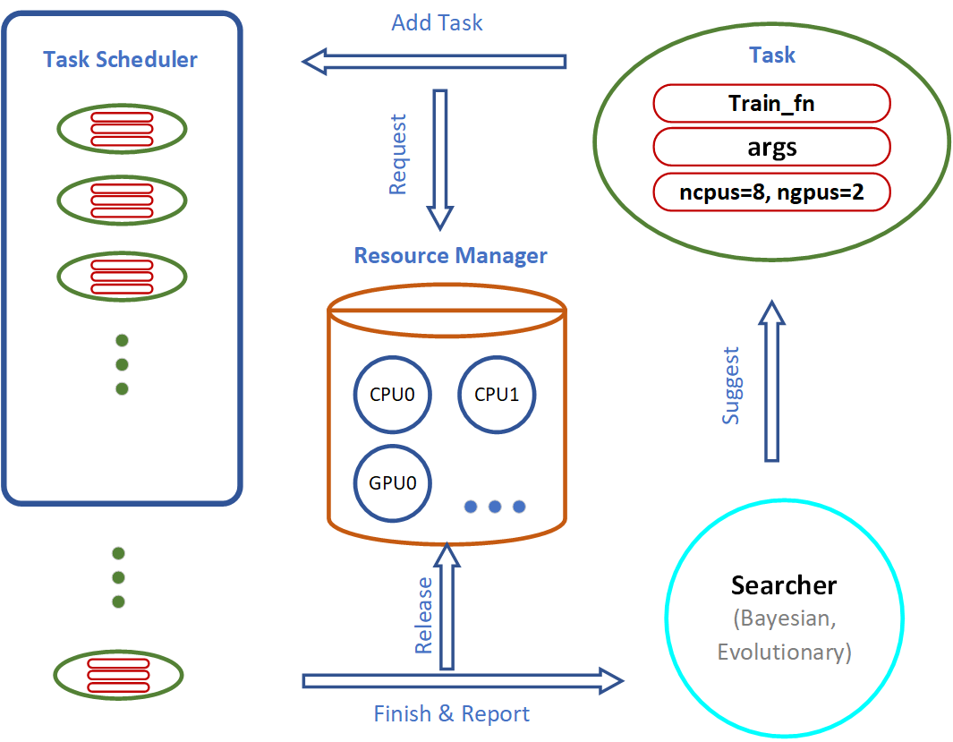
Important components of the AutoGluon system include the Searcher, Scheduler and Resource Manager:
The Searcher suggests hyperparameter configurations for the next training job.
The Scheduler runs the training job when computation resources become available.
In this tutorial, we illustrate how various search algorithms work and compare their performance via toy experiments.
FIFO Scheduling vs. Early Stopping
In this section, we compare the different behaviors of a sequential
First In, First Out (FIFO) scheduler using
autogluon.scheduler.FIFOScheduler vs. a preemptive scheduling
algorithm autogluon.scheduler.HyperbandScheduler that
early-terminates certain training jobs that do not appear promising
during their early stages.
Create a Dummy Training Function
import numpy as np
import autogluon as ag

@ag.args(
    lr=ag.space.Real(1e-3, 1e-2, log=True),
    wd=ag.space.Real(1e-3, 1e-2),
    epochs=10)
def train_fn(args, reporter):
    for e in range(args.epochs):
        dummy_accuracy = 1 - np.power(1.8, -np.random.uniform(e, 2*e))
        reporter(epoch=e+1, accuracy=dummy_accuracy, lr=args.lr, wd=args.wd)
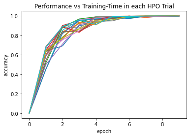
FIFO Scheduler
This scheduler runs training trials in order. When there are more resources available than required for a single training job, multiple training jobs may be run in parallel.
scheduler = ag.scheduler.FIFOScheduler(train_fn,
                                       resource={'num_cpus': 2, 'num_gpus': 0},
                                       num_trials=20,
                                       reward_attr='accuracy',
                                       time_attr='epoch')
scheduler.run()
scheduler.join_jobs()
/var/lib/jenkins/miniconda3/envs/autogluon_docs-v0_0_15/lib/python3.7/site-packages/ipykernel/ipkernel.py:287: DeprecationWarning: should_run_async will not call transform_cell automatically in the future. Please pass the result to transformed_cell argument and any exception that happen during thetransform in preprocessing_exc_tuple in IPython 7.17 and above.
  and should_run_async(code)
scheduler_options: Key 'searcher': Imputing default value random
scheduler_options: Key 'resume': Imputing default value False
scheduler_options: Key 'visualizer': Imputing default value none
scheduler_options: Key 'training_history_callback_delta_secs': Imputing default value 60
scheduler_options: Key 'delay_get_config': Imputing default value True

Starting Experiments
Num of Finished Tasks is 0
Num of Pending Tasks is 20
HBox(children=(HTML(value=''), FloatProgress(value=0.0, max=20.0), HTML(value='')))
Visualize the results:
scheduler.get_training_curves(plot=True, use_legend=False)
/var/lib/jenkins/miniconda3/envs/autogluon_docs-v0_0_15/lib/python3.7/site-packages/ipykernel/ipkernel.py:287: DeprecationWarning: should_run_async will not call transform_cell automatically in the future. Please pass the result to transformed_cell argument and any exception that happen during thetransform in preprocessing_exc_tuple in IPython 7.17 and above.
  and should_run_async(code)
Hyperband Scheduler
AutoGluon implements different variants of Hyperband scheduling, as
selected by type. In the stopping variant (the default), the
scheduler terminates training trials that don’t appear promising during
the early stages to free up compute resources for more promising
hyperparameter configurations.
scheduler = ag.scheduler.HyperbandScheduler(train_fn,
                                            resource={'num_cpus': 2, 'num_gpus': 0},
                                            num_trials=100,
                                            reward_attr='accuracy',
                                            time_attr='epoch',
                                            grace_period=1,
                                            reduction_factor=3,
                                            type='stopping')
scheduler.run()
scheduler.join_jobs()
max_t = 10, as inferred from train_fn.args
scheduler_options: Key 'resume': Imputing default value False
scheduler_options: Key 'brackets': Imputing default value 1
scheduler_options: Key 'keep_size_ratios': Imputing default value False
scheduler_options: Key 'maxt_pending': Imputing default value False
scheduler_options: Key 'searcher_data': Imputing default value rungs
scheduler_options: Key 'do_snapshots': Imputing default value False

scheduler_options: Key 'searcher': Imputing default value random
scheduler_options: Key 'visualizer': Imputing default value none
scheduler_options: Key 'training_history_callback_delta_secs': Imputing default value 60
scheduler_options: Key 'delay_get_config': Imputing default value True

Starting Experiments
Num of Finished Tasks is 0
Num of Pending Tasks is 100
HBox(children=(HTML(value=''), FloatProgress(value=0.0), HTML(value='')))
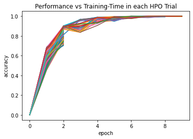
In this example, trials are stopped early after 1, 3, or 9 epochs. Only
a small fraction of the most promising jobs run for the full number of
10 epochs. Since the majority of trials are stopped early, we can afford
a larger num_trials. Visualize the results:
scheduler.get_training_curves(plot=True, use_legend=False)
Note that HyperbandScheduler needs to know the maximum number of
epochs. This can be passed as max_t argument. If it is missing (as
above), it is inferred from train_fn.args.epochs (which is set by
epochs=10 in the example above) or from train_fn.args.max_t
otherwise.
Random Search vs. Reinforcement Learning
In this section, we demonstrate the behaviors of random search and reinforcement learning in a simple simulation environment.
Create a Reward Function for Toy Experiments
Import the packages:
import matplotlib.pyplot as plt
from mpl_toolkits.mplot3d import Axes3D
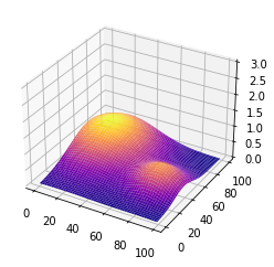
Input Space x = [0: 99], y = [0: 99]. The rewards is a combination
of 2 gaussians as shown in the following figure:
Generate the simulated reward as a mixture of 2 gaussians:
def gaussian2d(x, y, x0, y0, xalpha, yalpha, A):
    return A * np.exp( -((x-x0)/xalpha)**2 -((y-y0)/yalpha)**2)

x, y = np.linspace(0, 99, 100), np.linspace(0, 99, 100)
X, Y = np.meshgrid(x, y)

Z = np.zeros(X.shape)
ps = [(20, 70, 35, 40, 1),
      (80, 40, 20, 20, 0.7)]
for p in ps:
    Z += gaussian2d(X, Y, *p)
Visualize the reward space:
fig = plt.figure()
ax = fig.gca(projection='3d')
ax.plot_surface(X, Y, Z, cmap='plasma')
ax.set_zlim(0,np.max(Z)+2)
plt.show()
Create Training Function
We can simply define an AutoGluon searchable function with a decorator
ag.args. The reporter is used to communicate with AutoGluon
search and scheduling algorithms.
@ag.args(
    x=ag.space.Categorical(*list(range(100))),
    y=ag.space.Categorical(*list(range(100))),
)
def rl_simulation(args, reporter):
    x, y = args.x, args.y
    reporter(accuracy=Z[y][x])
Random Search
random_scheduler = ag.scheduler.FIFOScheduler(rl_simulation,
                                              resource={'num_cpus': 1, 'num_gpus': 0},
                                              num_trials=300,
                                              reward_attr="accuracy",
                                              resume=False)
random_scheduler.run()
random_scheduler.join_jobs()
print('Best config: {}, best reward: {}'.format(random_scheduler.get_best_config(), random_scheduler.get_best_reward()))
scheduler_options: Key 'searcher': Imputing default value random
scheduler_options: Key 'time_attr': Imputing default value epoch
scheduler_options: Key 'visualizer': Imputing default value none
scheduler_options: Key 'training_history_callback_delta_secs': Imputing default value 60
scheduler_options: Key 'delay_get_config': Imputing default value True

Starting Experiments
Num of Finished Tasks is 0
Num of Pending Tasks is 300
HBox(children=(HTML(value=''), FloatProgress(value=0.0, max=300.0), HTML(value='')))
Best config: {'x▁choice': 22, 'y▁choice': 69}, best reward: 0.9961362873852471
Reinforcement Learning
rl_scheduler = ag.scheduler.RLScheduler(rl_simulation,
                                        resource={'num_cpus': 1, 'num_gpus': 0},
                                        num_trials=300,
                                        reward_attr="accuracy",
                                        controller_batch_size=4,
                                        controller_lr=5e-3)
rl_scheduler.run()
rl_scheduler.join_jobs()
print('Best config: {}, best reward: {}'.format(rl_scheduler.get_best_config(), rl_scheduler.get_best_reward()))
scheduler_options: Key 'resume': Imputing default value False
scheduler_options: Key 'checkpoint': Imputing default value ./exp/checkpoint.ag
scheduler_options: Key 'ema_baseline_decay': Imputing default value 0.95
scheduler_options: Key 'controller_resource': Imputing default value {'num_cpus': 0, 'num_gpus': 0}
scheduler_options: Key 'sync': Imputing default value True

scheduler_options: Key 'time_attr': Imputing default value epoch
scheduler_options: Key 'visualizer': Imputing default value none
scheduler_options: Key 'training_history_callback_delta_secs': Imputing default value 60
scheduler_options: Key 'delay_get_config': Imputing default value True

Reserved DistributedResource(
    Node = Remote REMOTE_ID: 0,
    <Remote: 'inproc://172.31.38.222/9154/1' processes=1 threads=8, memory=33.24 GB>
    nCPUs = 0) in Remote REMOTE_ID: 0,
    <Remote: 'inproc://172.31.38.222/9154/1' processes=1 threads=8, memory=33.24 GB>
Starting Experiments
Num of Finished Tasks is 0
Num of Pending Tasks is 300
100%|██████████| 76/76 [00:19<00:00,  3.86it/s]
Best config: {'x▁choice': 21, 'y▁choice': 74}, best reward: 0.9892484241569526
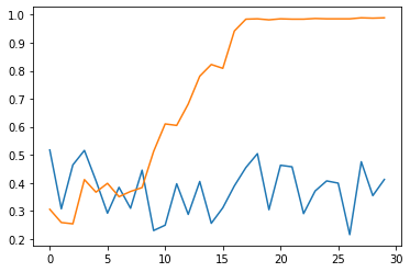
Compare the performance
Get the result history:
results_rl = [v[0]['accuracy'] for v in rl_scheduler.training_history.values()]
results_random = [v[0]['accuracy'] for v in random_scheduler.training_history.values()]
Average result every 10 trials:
import statistics
results1 = [statistics.mean(results_random[i:i+10]) for i in range(0, len(results_random), 10)]
results2 = [statistics.mean(results_rl[i:i+10]) for i in range(0, len(results_rl), 10)]
Plot the results:
plt.plot(range(len(results1)), results1, range(len(results2)), results2)
[<matplotlib.lines.Line2D at 0x7fa0203f4c50>,
 <matplotlib.lines.Line2D at 0x7fa0204f6f90>]