Forecasting with Chronos-2
![]()

AutoGluon-TimeSeries (AG-TS) includes the Chronos family of forecasting models. Chronos models are pretrained on a large collection of real and synthetic time series data, enabling accurate out-of-the-box forecasts on new data.
AG-TS provides a robust and user-friendly way to work with Chronos through the familiar TimeSeriesPredictor API. It allows users to backtest models, compare them with other forecasting approaches, and ensemble Chronos with other models to build robust forecasting pipelines. This tutorial demonstrates how to:
Use Chronos-2 in zero-shot mode to generate forecasts without dataset-specific training
Fine-tune Chronos-2 on custom data to improve accuracy
Tip
This tutorial shows how to run Chronos-2 on your own machine. For production use on AWS, check out AutoGluon-Cloud — deploy Chronos-2 to run real-time, serverless, or batch inference on Amazon SageMaker using the same familiar API.
Getting started with Chronos-2
Being a pretrained model for zero-shot forecasting, Chronos is different from other models available in AG-TS.
Specifically, by default, Chronos models do not really fit time series data. However, when predict is called, they perform zero-shot inference by using the provided contextual information. In this aspect, they behave like local statistical models such as ETS or ARIMA, where all computation happens during inference.
AutoGluon supports the original Chronos models (e.g., chronos-t5-large), the Chronos-Bolt models (e.g., chronos-bolt-base), and the latest Chronos-2 models (e.g., chronos-2). The following table compares the capabilities of the three model families.
Capability |
Chronos |
Chronos-Bolt |
Chronos-2 |
|---|---|---|---|
Univariate Forecasting |
✅ |
✅ |
✅ |
Cross-learning across items |
❌ |
❌ |
✅ |
Multivariate Forecasting |
❌ |
❌ |
✅ |
Past-only (real/categorical) covariates |
❌ |
❌ |
✅ |
Known future (real/categorical) covariates |
🧩 |
🧩 |
✅ |
Fine-tuning support |
✅ |
✅ |
✅ |
Max. Context Length |
512 |
2048 |
8192 |
Max. Prediction Length |
64 |
64 |
1024 |
The easiest way to get started with Chronos is through the model-specific presets.
(recommended) The Chronos-2 models can be accessed using the
"chronos2_small"and"chronos2"presets.The Chronos-Bolt️ models can be accessed using the
"bolt_tiny","bolt_mini","bolt_small"and"bolt_base"presets.
Alternatively, Chronos models can be combined with other time series models using presets "medium_quality", "high_quality" and "best_quality". More details about these presets are available in the documentation for TimeSeriesPredictor.fit.
🧩 Chronos/Chronos-Bolt do not natively support future covariates, but they can be combined with external covariate regressors. This only models per-timestep effects, not effects across time. In contrast, Chronos-2 supports all covariate types natively.
Zero-shot forecasting
Univariate Forecasting
Let’s work with a subset of the Australian Electricity Demand dataset to see Chronos-2 in action.
First, we load the dataset as a TimeSeriesDataFrame.
import pandas as pd
from autogluon.timeseries import TimeSeriesDataFrame, TimeSeriesPredictor
data = TimeSeriesDataFrame.from_path(
    "https://autogluon.s3.amazonaws.com/datasets/timeseries/australian_electricity_subset/test.csv"
)
data.head()
| target | ||
|---|---|---|
| item_id | timestamp | |
| T000000 | 2013-03-10 00:00:00 | 5207.959961 |
| 2013-03-10 00:30:00 | 5002.275879 | |
| 2013-03-10 01:00:00 | 4747.569824 | |
| 2013-03-10 01:30:00 | 4544.880859 | |
| 2013-03-10 02:00:00 | 4425.952148 |
Next, we create the TimeSeriesPredictor and select the "chronos2" presets to use the Chronos-2 (120M) model in zero-shot mode.
num_test_windows = 3
prediction_length = 48
train_data, test_data = data.train_test_split(num_test_windows * prediction_length)

predictor = TimeSeriesPredictor(prediction_length=prediction_length).fit(
    train_data,
    presets="chronos2",
)
As promised, Chronos does not take any time to fit. The fit call merely serves as a proxy for the TimeSeriesPredictor to do some of its chores under the hood, such as inferring the frequency of time series and saving the predictor’s state to disk.
Let’s use the predict method to generate forecasts.
predictions = predictor.predict(train_data)
predictions.head()
Model not specified in predict, will default to the model with the best validation score: Chronos2
| mean | 0.1 | 0.2 | 0.3 | 0.4 | 0.5 | 0.6 | 0.7 | 0.8 | 0.9 | ||
|---|---|---|---|---|---|---|---|---|---|---|---|
| item_id | timestamp | ||||||||||
| T000000 | 2015-02-26 00:00:00 | 5223.812012 | 5153.143066 | 5178.589355 | 5193.954102 | 5210.103027 | 5223.812012 | 5234.564453 | 5248.638672 | 5265.144531 | 5295.290527 |
| 2015-02-26 00:30:00 | 5001.890625 | 4940.849609 | 4967.337891 | 4982.128906 | 4991.323242 | 5001.890625 | 5012.041504 | 5026.311523 | 5047.328125 | 5078.305664 | |
| 2015-02-26 01:00:00 | 4759.131348 | 4684.923340 | 4712.408691 | 4729.203125 | 4743.586426 | 4759.131348 | 4770.625977 | 4784.588379 | 4803.948242 | 4828.079590 | |
| 2015-02-26 01:30:00 | 4560.188477 | 4505.166016 | 4523.577637 | 4535.824219 | 4550.487793 | 4560.188477 | 4580.131348 | 4591.911621 | 4615.944336 | 4636.415039 | |
| 2015-02-26 02:00:00 | 4439.416992 | 4369.610352 | 4390.421875 | 4412.242676 | 4428.110352 | 4439.416992 | 4456.724609 | 4474.257324 | 4496.028320 | 4509.392090 |
We get a dataframe with the point forecast (mean) and nine quantiles which capture the uncertainty in the forecasts. Custom quantile levels can be specified as follows:
TimeSeriesPredictor(..., quantile_levels=[0.05, 0.1, 0.5, 0.9, 0.95])
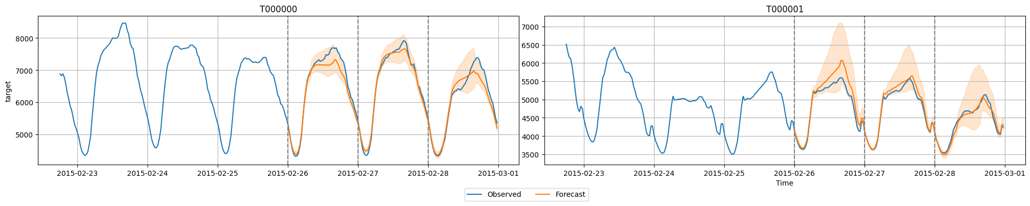
AG-TS also makes it easy to generate predictions for multiple backtest dates and to visualize the models’ predictions.
import matplotlib.pyplot as plt

# Generate predictions for multiple windows
predictions_per_window = predictor.backtest_predictions(test_data, num_val_windows=num_test_windows)

# Plot predictions for the first two time series
item_ids = test_data.item_ids[:2].tolist()
all_predictions = pd.concat(predictions_per_window)
predictor.plot(test_data, all_predictions, max_history_length=300, item_ids=item_ids)

# Optional: Plot the cutoff dates with dashed vertical lines
for cutoff in range(-num_test_windows * prediction_length, 0, prediction_length):
    for i, ax in enumerate(plt.gcf().axes):
        cutoff_timestamp = test_data.loc[item_ids[i]].index[cutoff]
        ax.axvline(cutoff_timestamp, color='gray', linestyle='--')
plt.show()
Forecasting with covariates
The previous example showed Chronos-2 in action on a univariate forecasting task, i.e., only the historical data of the target time series for making predictions. However, in real-world scenarios, additional exogenous information related to the target series (e.g., weather forecasts, holidays, promotions) is often available. These exogenous time series, often referred to as covariates, may either be observed only in the past (past-only) or also in the forecast horizon (known future). Leveraging this information when making predictions can improve forecast accuracy.
Chronos-2 natively supports (dynamic) covariates, past-only and known-future, real-valued or categorical. Let’s see how we can use Chronos-2 to forecast with covariates on a Electrical Load Forecasting task.
data = TimeSeriesDataFrame.from_path(
    "https://autogluon.s3.amazonaws.com/datasets/timeseries/bull/test.parquet", id_column="id"
)
data.head()
| load | airtemperature | dewtemperature | sealvlpressure | ||
|---|---|---|---|---|---|
| item_id | timestamp | ||||
| Bull_education_Magaret | 2016-01-01 00:00:00 | 0.0000 | 9.4 | 3.3 | 1028.699951 |
| 2016-01-01 01:00:00 | 2.7908 | 8.9 | 2.2 | 1028.800049 | |
| 2016-01-01 02:00:00 | 3.7210 | 8.9 | 2.2 | 1029.599976 | |
| 2016-01-01 03:00:00 | 2.7908 | 8.3 | 1.7 | 1029.500000 | |
| 2016-01-01 04:00:00 | 9.3025 | 7.8 | 1.7 | 1029.599976 |
The goal is to forecast next day’s (24 hours) load using historical load and known weather covariates: air temperature, dew temperature and sea level pressure. Since future weather information is not known in advance, weather forecasts are typically used as known covariates.
prediction_length = 24
train_data, test_data = data.train_test_split(prediction_length=prediction_length)
Sorting the dataframe index before generating the train/test split.
The following code uses Chronos-2 in the TimeSeriesPredictor to forecast the load for the next 24 hours. We use the univariate Chronos-Bolt (Small) model as a baseline for comparison.
Note that we have specified the target column we are interested in forecasting and the names of known covariates while constructing the TimeSeriesPredictor. Any other columns, if present, will be used as past-only covariates.
predictor = TimeSeriesPredictor(
    prediction_length=prediction_length,
    target="load",
    known_covariates_names=["airtemperature", "dewtemperature", "sealvlpressure"],
    eval_metric="MASE",
).fit(
    train_data,
    hyperparameters={"Chronos": {}, "Chronos2": {}},
    enable_ensemble=False,
    time_limit=60,
)
Once the predictor has been fit, we can evaluate it on the test dataset and generate the leaderboard. We see that Chronos-2, which utilizes covariates, produces a significantly more accurate forecast on the test set compared to Chronos-Bolt, which does not utilize covariates.
Note that all AutoGluon-TimeSeries models report scores in a “higher is better” format, meaning that most forecasting error metrics like MASE are multiplied by -1 when reported.
predictor.leaderboard(test_data)
Additional data provided, testing on additional data. Resulting leaderboard will be sorted according to test score (`score_test`).
| model | score_test | score_val | pred_time_test | pred_time_val | fit_time_marginal | fit_order | |
|---|---|---|---|---|---|---|---|
| 0 | Chronos2 | -0.696239 | -0.817203 | 6.869672 | 6.662584 | 0.568715 | 1 |
| 1 | Chronos[autogluon__chronos-bolt-small] | -1.278404 | -1.086471 | 0.303209 | 0.354011 | 0.571351 | 2 |
We can also use the predictor to compute features importances to understand which exogenous features are affecting the prediction accuracy the most.
predictor.feature_importance(test_data, model="Chronos2", relative_scores=True)
Computing feature importance
| importance | stdev | n | p99_low | p99_high | |
|---|---|---|---|---|---|
| airtemperature | 0.324308 | 0.000000e+00 | 5.0 | 0.324308 | 0.324308 |
| dewtemperature | 0.057110 | 7.757919e-18 | 5.0 | 0.057110 | 0.057110 |
| sealvlpressure | 0.038278 | 0.000000e+00 | 5.0 | 0.038278 | 0.038278 |
With relative_scores=True, this method returns relative (percentage) improvements in the eval_metric due to each feature. In this example, the airtemperature feature is the most important for accurate forecasting, yielding a ~32% error reduction on the test set.
Note that covariates may not always be useful and using more covariates does not necessarily imply more accurate forecasts. With Chronos-2, AutoGluon makes it easy for users to quickly validate different configurations and find ones that perform best on held-out data.
Fine-tuning
We have seen above how Chronos-2 models can produce forecasts in zero-shot mode, both with and without covariates. AutoGluon also makes it easy to fine-tune Chronos models on a specific dataset to maximize the predictive accuracy.
The following snippet specifies two settings for the Chronos-2 model: zero-shot and fine-tuned. TimeSeriesPredictor will perform a lightweight fine-tuning of the pretrained model on the provided training data. We add name suffixes to easily identify the zero-shot and fine-tuned versions of the model.
Note
If you are fine-tuning on a machine with multiple GPUs, we strongly recommend setting the CUDA_VISIBLE_DEVICES environment variable to ensure that only a single GPU is visible.
predictor = TimeSeriesPredictor(
    prediction_length=prediction_length,
    target="load",
    known_covariates_names=["airtemperature", "dewtemperature", "sealvlpressure"],
    eval_metric="MASE",
).fit(
    train_data=train_data,
    hyperparameters={
        "Chronos2": [
            # Zero-shot model
            {"ag_args": {"name_suffix": "ZeroShot"}},
            # Fine-tuned model
            {"fine_tune": True, "ag_args": {"name_suffix": "FineTuned"}},
        ]
    },
    time_limit=300,  # time limit in seconds
    enable_ensemble=False,
)
Here we used the default fine-tuning configuration for Chronos-2 by only specifying "fine_tune": True. By default, Chronos-2 is fine-tuned with a low-rank adapter (LoRA) to reduce memory and disk footprint. AutoGluon makes it easy to change other parameters for fine-tuning such as the mode, number of steps or learning rate.
predictor.fit(
    ...,
    hyperparameters={"Chronos2": {"fine_tune": True, "fine_tune_mode": "full", "fine_tune_lr": 1e-4, "fine_tune_steps": 2000, "fine_tune_batch_size": 32}},
)
For the full list of fine-tuning options, see the Chronos-2 documentation in Forecasting Model Zoo.
After fitting, we can evaluate the two model variants on the test data and generate a leaderboard.
predictor.leaderboard(test_data)
Additional data provided, testing on additional data. Resulting leaderboard will be sorted according to test score (`score_test`).
| model | score_test | score_val | pred_time_test | pred_time_val | fit_time_marginal | fit_order | |
|---|---|---|---|---|---|---|---|
| 0 | Chronos2FineTuned | -0.689780 | -0.819946 | 7.199853 | 7.966381 | 267.469054 | 2 |
| 1 | Chronos2ZeroShot | -0.696239 | -0.817203 | 7.000247 | 6.647804 | 0.573972 | 1 |
Fine-tuning resulted in a more accurate model, as shown by the better score_test on the test set.
FAQ
How accurate is Chronos-2?
Chronos-2 is the best performing (last updated: Dec 2025) time series foundation model across multiple benchmarks, including fev-bench, GIFT-Eval and Chronos Bench II. Details empirical results can be found in the Chronos-2 technical report. The accuracy of Chronos-2 often exceeds statistical baseline models and task-specific deep learning models such as DeepAR and TemporalFusionTransformer.
Does fine-tuning always improve Chronos-2’s forecasting accuracy?
Fine-tuning a foundation model like Chronos-2 involves many hyperparameter choices. AG-TS provides reasonable defaults that performed well in large-scale benchmarking, but they may not be optimal for every use case. We recommend fine-tuning only when you have a reasonable number of time series and sufficient historical data (e.g., >100 time series with a median history length larger than 3 * prediction_length), as limited data can lead to overfitting or degraded performance. If you observe degraded accuracy, we recommend increasing the size of the training data and experimenting with different fine-tuning hyperparameters.
Alternatively, you can use an ensemble of zero-shot Chronos-2 and fine-tuned Chronos-2 (Small) to construct a robust predictor, available via the chronos2_ensemble preset:
predictor = TimeSeriesPredictor(prediction_length=prediction_length).fit(
    ...,
    presets="chronos2_ensemble",
)
What is the recommended hardware for running Chronos models?
We recommend using a machine with a GPU for best performance, especially for fine-tuning. For reference, we tested the models on AWS g5.2xlarge instances with NVIDIA A10G GPUs (24 GiB GPU memory) and 32 GiB of system memory. However, Chronos-2, Chronos-Bolt, and Chronos (up to small size) can also run on consumer GPUs and CPUs with reasonable inference times.
Why do my predictions change with the batch_size?
By default, AutoGluon enables Chronos-2’s cross_learning mode, where the model makes joint predictions across time series within a batch. This often improves accuracy but also makes results sensitive to the batch_size. You can disable this mode with:
predictor.fit(
    ...,
    hyperparameters={"Chronos2": {"cross_learning": False}},
)
Where can I ask specific questions on Chronos?
Members of the AutoGluon team are among the core developers of Chronos. So you can ask Chronos-related questions on AutoGluon’s GitHub or on Chronos’ GitHub.