AutoMM Detection - Finetune on COCO Format Dataset with Customized Settings


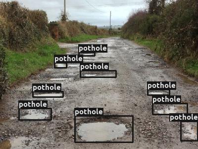
In this section, our goal is to fast finetune and evaluate a pretrained model
on Pothole dataset in COCO format with customized setting.
Pothole is a single object, i.e. pothole, detection dataset, containing 665 images with bounding box annotations
for the creation of detection models and can work as POC/POV for the maintenance of roads.
See AutoMM Detection - Prepare Pothole Dataset for how to prepare Pothole dataset.
To start, make sure mmcv and mmdet are installed.
Note: MMDet is no longer actively maintained and is only compatible with MMCV version 2.1.0. Installation can be problematic due to CUDA version compatibility issues. For best results:
Use CUDA 12.4 with PyTorch 2.5
Before installation, run:
pip install -U pip setuptools wheel
sudo apt-get install -y ninja-build gcc g++
This will help prevent MMCV installation from hanging during wheel building.
After installation in Jupyter notebook, restart the kernel for changes to take effect.
# Update package tools and install build dependencies
!pip install -U pip setuptools wheel
!sudo apt-get install -y ninja-build gcc g++

# Install MMCV
!python3 -m mim install "mmcv==2.1.0"

# For Google Colab users: If the above fails, use this alternative MMCV installation
# pip install "mmcv==2.1.0" -f https://download.openmmlab.com/mmcv/dist/cu121/torch2.1.0/index.html

# Install MMDet
!python3 -m pip install "mmdet==3.2.0"

# Install MMEngine (version >=0.10.6 for PyTorch 2.5 compatibility)
!python3 -m pip install "mmengine>=0.10.6"
from autogluon.multimodal import MultiModalPredictor
/home/ci/opt/venv/lib/python3.13/site-packages/tqdm/auto.py:21: TqdmWarning: IProgress not found. Please update jupyter and ipywidgets. See https://ipywidgets.readthedocs.io/en/stable/user_install.html
  from .autonotebook import tqdm as notebook_tqdm
---------------------------------------------------------------------------
ModuleNotFoundError                       Traceback (most recent call last)
Cell In[3], line 1
----> 1 from autogluon.multimodal import MultiModalPredictor

File ~/autogluon/multimodal/src/autogluon/multimodal/__init__.py:8
      5 except ImportError:
      6     pass
----> 8 from .predictor import MultiModalPredictor
     10 _add_stream_handler()

File ~/autogluon/multimodal/src/autogluon/multimodal/predictor.py:19
     16 from autogluon.core.metrics import Scorer
     18 from .constants import AUTOMM_TUTORIAL_MODE, FEW_SHOT_CLASSIFICATION, NER, OBJECT_DETECTION, SEMANTIC_SEGMENTATION
---> 19 from .learners import (
     20     BaseLearner,
     21     EnsembleLearner,
     22     FewShotSVMLearner,
     23     MatchingLearner,
     24     NERLearner,
     25     ObjectDetectionLearner,
     26     SemanticSegmentationLearner,
     27 )
     28 from .utils import get_dir_ckpt_paths
     29 from .utils.problem_types import PROBLEM_TYPES_REG

File ~/autogluon/multimodal/src/autogluon/multimodal/learners/__init__.py:1
----> 1 from .base import BaseLearner
      2 from .ensemble import EnsembleLearner
      3 from .few_shot_svm import FewShotSVMLearner

File ~/autogluon/multimodal/src/autogluon/multimodal/learners/base.py:71
     31 from .. import version as ag_version
     32 from ..constants import (
     33     BEST,
     34     BEST_K_MODELS_FILE,
   (...)     69     ZERO_SHOT_IMAGE_CLASSIFICATION,
     70 )
---> 71 from ..data import (
     72     BaseDataModule,
     73     MultiModalFeaturePreprocessor,
     74     create_fusion_data_processors,
     75     data_to_df,
     76     get_mixup,
     77     infer_column_types,
     78     infer_dtypes_by_model_names,
     79     infer_output_shape,
     80     infer_problem_type,
     81     infer_scarcity_mode_by_data_size,
     82     init_df_preprocessor,
     83     is_image_column,
     84     split_train_tuning_data,
     85     turn_on_off_feature_column_info,
     86 )
     87 from ..models import (
     88     create_fusion_model,
     89     get_model_postprocess_fn,
   (...)     92     select_model,
     93 )
     94 from ..optim import (
     95     compute_score,
     96     get_aug_loss_func,
   (...)    103     infer_metrics,
    104 )

File ~/autogluon/multimodal/src/autogluon/multimodal/data/__init__.py:1
----> 1 from .datamodule import BaseDataModule
      2 from .dataset import BaseDataset
      3 from .dataset_mmlab import MultiImageMixDataset

File ~/autogluon/multimodal/src/autogluon/multimodal/data/datamodule.py:8
      5 from torch.utils.data import DataLoader, Dataset
      7 from ..constants import PREDICT, TEST, TRAIN, VALIDATE
----> 8 from .dataset import BaseDataset
      9 from .preprocess_dataframe import MultiModalFeaturePreprocessor
     10 from .utils import get_collate_fn

File ~/autogluon/multimodal/src/autogluon/multimodal/data/dataset.py:9
      7 from ..constants import GET_ITEM_ERROR_RETRY
      8 from .preprocess_dataframe import MultiModalFeaturePreprocessor
----> 9 from .utils import apply_data_processor, apply_df_preprocessor, get_per_sample_features
     11 logger = logging.getLogger(__name__)
     14 class BaseDataset(torch.utils.data.Dataset):

File ~/autogluon/multimodal/src/autogluon/multimodal/data/utils.py:48
     46 from .process_numerical import NumericalProcessor
     47 from .process_semantic_seg_img import SemanticSegImageProcessor
---> 48 from .process_text import TextProcessor
     50 logger = logging.getLogger(__name__)
     53 def get_collate_fn(
     54     df_preprocessor: Union[MultiModalFeaturePreprocessor, List[MultiModalFeaturePreprocessor]],
     55     data_processors: Union[Dict, List[Dict]],
     56     per_gpu_batch_size: Optional[int] = None,
     57 ):

File ~/autogluon/multimodal/src/autogluon/multimodal/data/process_text.py:19
     17 from ..models.utils import get_pretrained_tokenizer
     18 from .collator import PadCollator, StackCollator
---> 19 from .template_engine import TemplateEngine
     20 from .trivial_augmenter import TrivialAugment
     22 logger = logging.getLogger(__name__)

File ~/autogluon/multimodal/src/autogluon/multimodal/data/template_engine.py:6
      3 import numpy as np
      4 from omegaconf import DictConfig, OmegaConf
----> 6 from .templates import DatasetTemplates, Template, TemplateCollection
      8 logger = logging.getLogger(__name__)
     11 class TemplateEngine:

File ~/autogluon/multimodal/src/autogluon/multimodal/data/templates.py:16
     13 from typing import Dict, List, Optional, Tuple
     15 import pandas as pd
---> 16 import pkg_resources
     17 import yaml
     18 from jinja2 import BaseLoader, Environment, meta

ModuleNotFoundError: No module named 'pkg_resources'
And also import some other packages that will be used in this tutorial:
import os

from autogluon.core.utils.loaders import load_zip
We have the sample dataset ready in the cloud. Let’s download it and store the paths for each data split:
zip_file = "https://automl-mm-bench.s3.amazonaws.com/object_detection/dataset/pothole.zip"
download_dir = "./pothole"

load_zip.unzip(zip_file, unzip_dir=download_dir)
data_dir = os.path.join(download_dir, "pothole")
train_path = os.path.join(data_dir, "Annotations", "usersplit_train_cocoformat.json")
val_path = os.path.join(data_dir, "Annotations", "usersplit_val_cocoformat.json")
test_path = os.path.join(data_dir, "Annotations", "usersplit_test_cocoformat.json")
While using COCO format dataset, the input is the json annotation file of the dataset split.
In this example, usersplit_train_cocoformat.json is the annotation file of the train split.
usersplit_val_cocoformat.json is the annotation file of the validation split.
And usersplit_test_cocoformat.json is the annotation file of the test split.
We select the YOLOX-small model pretrained on COCO dataset. With this setting, it is fast to finetune or inference,
and easy to deploy. Note that you can use a larger model by setting the checkpoint_name to corresponding checkpoint name for better performance (but usually with slower speed).
And you may need to change the lr and per_gpu_batch_size for a different model.
An easier way is to use our predefined presets "medium_quality", "high_quality", or "best_quality".
For more about using presets, see Quick Start Coco.
checkpoint_name = "yolox_s"
num_gpus = 1  # only use one GPU
We create the MultiModalPredictor with selected checkpoint name and number of GPUs.
We need to specify the problem_type to "object_detection",
and also provide a sample_data_path for the predictor to infer the categories of the dataset.
Here we provide the train_path, and it also works using any other split of this dataset.
predictor = MultiModalPredictor(
    hyperparameters={
        "model.mmdet_image.checkpoint_name": checkpoint_name,
        "env.num_gpus": num_gpus,
    },
    problem_type="object_detection",
    sample_data_path=train_path,
)
We set the learning rate to be 1e-4.
Note that we use a two-stage learning rate option during finetuning by default,
and the model head will have 100x learning rate.
Using a two-stage learning rate with high learning rate only on head layers makes
the model converge faster during finetuning. It usually gives better performance as well,
especially on small datasets with hundreds or thousands of images.
We set batch size to be 16, and you can increase or decrease the batch size based on your available GPU memory.
We set max number of epochs to 30, number of validation check per interval to 1.0,
and validation check per n epochs to 3 for fast finetuning.
We also compute the time of the fit process here for better understanding the speed.
predictor.fit(
    train_path,
    tuning_data=val_path,
    hyperparameters={
        "optim.lr": 1e-4,  # we use two stage and detection head has 100x lr
        "env.per_gpu_batch_size": 16,  # decrease it when model is large or GPU memory is small
        "optim.max_epochs": 30,  # max number of training epochs, note that we may early stop before this based on validation setting
        "optim.val_check_interval": 1.0,  # Do 1 validation each epoch
        "optim.check_val_every_n_epoch": 3,  # Do 1 validation each 3 epochs
        "optim.patience": 3,  # Early stop after 3 consective validations are not the best
    },
)
To evaluate the model we just trained, run:
predictor.evaluate(test_path)
Note that it’s always recommended to use our predefined presets to save customization time with following code script:
predictor = MultiModalPredictor(
    problem_type="object_detection",
    sample_data_path=train_path,
    presets="medium_quality",
)
predictor.fit(train_path, tuning_data=val_path)
predictor.evaluate(test_path)
For more about using presets, see Quick Start Coco.
And the evaluation results are shown in command line output. The first value is mAP in COCO standard, and the second one is mAP in VOC standard (or mAP50). For more details about these metrics, see COCO’s evaluation guideline.
We can get the prediction on test set:
pred = predictor.predict(test_path)
Let’s also visualize the prediction result:
!pip install opencv-python
from autogluon.multimodal.utils import visualize_detection
conf_threshold = 0.25  # Specify a confidence threshold to filter out unwanted boxes
visualization_result_dir = "./"  # Use the pwd as result dir to save the visualized image
visualized = visualize_detection(
    pred=pred[12:13],
    detection_classes=predictor.classes,
    conf_threshold=conf_threshold,
    visualization_result_dir=visualization_result_dir,
)
from PIL import Image
from IPython.display import display
img = Image.fromarray(visualized[0][:, :, ::-1], 'RGB')
display(img)
Under this fast finetune setting, we reached a good mAP number on a new dataset with a few hundred seconds!
For how to finetune with higher performance,
see AutoMM Detection - High Performance Finetune on COCO Format Dataset, where we finetuned a VFNet model with
5 hours and reached mAP = 0.450, mAP50 = 0.718 on this dataset.
Other Examples
You may go to AutoMM Examples to explore other examples about AutoMM.
Customization
To learn how to customize AutoMM, please refer to Customize AutoMM.
Citation
@article{DBLP:journals/corr/abs-2107-08430,
  author    = {Zheng Ge and
               Songtao Liu and
               Feng Wang and
               Zeming Li and
               Jian Sun},
  title     = {{YOLOX:} Exceeding {YOLO} Series in 2021},
  journal   = {CoRR},
  volume    = {abs/2107.08430},
  year      = {2021},
  url       = {https://arxiv.org/abs/2107.08430},
  eprinttype = {arXiv},
  eprint    = {2107.08430},
  timestamp = {Tue, 05 Apr 2022 14:09:44 +0200},
  biburl    = {https://dblp.org/rec/journals/corr/abs-2107-08430.bib},
  bibsource = {dblp computer science bibliography, https://dblp.org},
}