Anomaly Detection Analysis

Anomaly detection is a powerful technique used in data analysis and machine learning to identify unusual patterns or behaviors that deviate from the norm. These deviations, known as anomalies or outliers, can be indicative of errors, fraud, system failures, or other exceptional events. By detecting these anomalies early, organizations can take proactive measures to address potential issues, enhance security, optimize processes, and make more informed decisions. In this tutorial, we will introduce anomaly detection tools available in AutoGluon EDA package and showcase how to identify these irregularities within your data, even if you’re new to the subject.

import pandas as pd
import seaborn as sns

import autogluon.eda.auto as auto

Loading and pre-processing the data

First we will load the data. We will use the Titanic dataset.

df_train = pd.read_csv('https://autogluon.s3.amazonaws.com/datasets/titanic/train.csv')
df_test = pd.read_csv('https://autogluon.s3.amazonaws.com/datasets/titanic/test.csv')
target_col = 'Survived'

auto.detect_anomalies will automatically preprocess the data, but it doesn’t fill in missing numeric values by default. We’ll take care of filling those in ourselves before feeding the data into the anomaly detector.

x = df_train
x_test = df_test
x.Age.fillna(x.Age.mean(), inplace=True)
x_test.Age.fillna(x.Age.mean(), inplace=True)
x_test.Fare.fillna(x.Fare.mean(), inplace=True)

Running Initial Anomaly Analysis

# This parameter specifies how many standard deviations above mean anomaly score are considered
# to be anomalies (only needed for visualization, does not affect scores calculation).
threshold_stds = 3

auto.detect_anomalies(
    train_data=x,
    test_data=x_test,
    label=target_col,
    threshold_stds=threshold_stds,
    show_top_n_anomalies=None,
    fig_args={
        'figsize': (6, 4)
    },
    chart_args={
        'normal.color': 'lightgrey',
        'anomaly.color': 'orange',
    }
)

Anomaly Detection Report

When interpreting anomaly scores, consider:

• Threshold: Determine a suitable threshold to separate normal from anomalous data points, based on domain knowledge or statistical methods.

• Context: Examine the context of anomalies, including time, location, and surrounding data points, to identify possible causes.

• False positives/negatives: Be aware of the trade-offs between false positives (normal points classified as anomalies) and false negatives (anomalies missed).

• Feature relevance: Ensure the features used for anomaly detection are relevant and contribute to the model’s performance.

• Model performance: Regularly evaluate and update the model to maintain its accuracy and effectiveness.

It’s important to understand the context and domain knowledge before deciding on an appropriate approach to deal with anomalies.The choice of method depends on the data’s nature, the cause of anomalies, and the problem being addressed.The common ways to deal with anomalies:

• Removal: If an anomaly is a result of an error, noise, or irrelevance to the analysis, it can be removed from the dataset to prevent it from affecting the model’s performance.

• Imputation: Replace anomalous values with appropriate substitutes, such as the mean, median, or mode of the feature, or by using more advanced techniques like regression or k-nearest neighbors.

• Transformation: Apply transformations like log, square root, or z-score to normalize the data and reduce the impact of extreme values. Absolute dates might be transformed into relative features like age of the item.

• Capping: Set upper and lower bounds for a feature, and replace values outside these limits with the bounds themselves. This method is also known as winsorizing.

• Separate modeling: Treat anomalies as a distinct group and build a separate model for them, or use specialized algorithms designed for handling outliers, such as robust regression or one-class SVM.

• Incorporate as a feature: Create a new binary feature indicating the presence of an anomaly, which can be useful if anomalies have predictive value.

_{^{Use show_help_text=False to hide this information when calling this function.}}

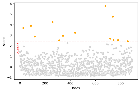
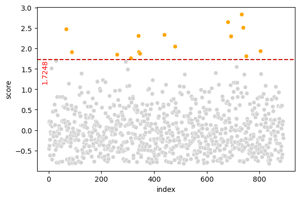
train_data anomalies for 3-sigma outlier scores

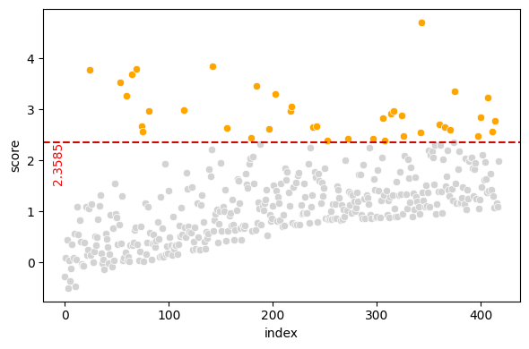
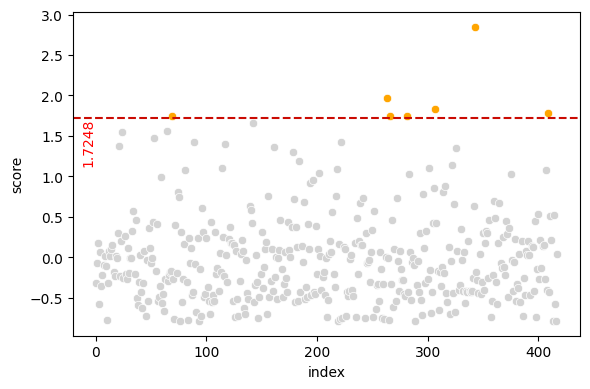
test_data anomalies for 3-sigma outlier scores

Handling Covariate Shift

The test data chart appears to show increasing anomaly scores as we move through the records. This is not normal; let’s check for a covariate shift.

auto.covariate_shift_detection(train_data=x, test_data=x_test, label=target_col)

We detected a substantial difference between the training and test X distributions, a type of distribution shift.

Test results: We can predict whether a sample is in the test vs. training set with a roc_auc of 0.9999 with a p-value of 0.0010 (smaller than the threshold of 0.0100).

Feature importances: The variables that are the most responsible for this shift are those with high feature importance:

	importance	stddev	p_value	n	p99_high	p99_low
PassengerId	0.480003	0.031567	0.000002	5	0.545000	0.415006
Name	0.000167	0.000091	0.007389	5	0.000355	-0.000020

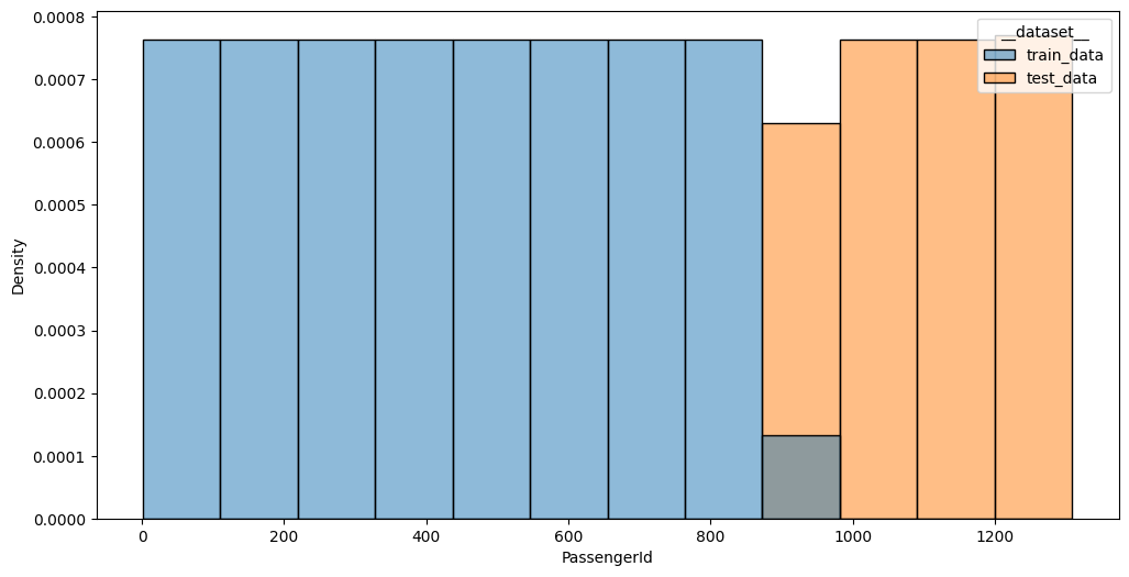
PassengerId values distribution between datasets; p-value: 0.0000

ax = sns.lineplot(data=df_train[['PassengerId']].reset_index(), x='index', y='PassengerId', label='Train')
sns.lineplot(ax=ax, data=df_test[['PassengerId']].reset_index(), x='index', y='PassengerId', label='Test');

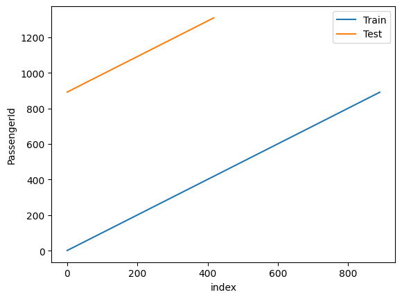
This feature looks like a monotonically increasing ID and carries no value for our problem; we are going to remove it.

x = x.drop(columns=['PassengerId'], errors='ignore')
x_test = x_test.drop(columns=['PassengerId'], errors='ignore')

auto.covariate_shift_detection(train_data=x, test_data=x_test, label=target_col)

We did not detect a substantial difference between the training and test X distributions.

Run Anomaly Analysis on Cleaned Data

state = auto.detect_anomalies(
    train_data=x,
    test_data=x_test,
    label=target_col,
    threshold_stds=3,
    show_top_n_anomalies=5,
    explain_top_n_anomalies=1,
    return_state=True,
    show_help_text=False,
    fig_args={
        'figsize': (6, 4)
    },
    chart_args={
        'normal.color': 'lightgrey',
        'anomaly.color': 'orange',
    }    
)

Anomaly Detection Report

train_data anomalies for 3-sigma outlier scores

test_data anomalies for 3-sigma outlier scores

Top-5 train_data anomalies (total: 15)

	Survived	Pclass	Name	Sex	Age	SibSp	Parch	Ticket	Fare	Cabin	Embarked	score
732	0	2	Knight, Mr. Robert J	male	29.699118	0	0	239855	0.0000	NaN	S	2.827401
679	1	1	Cardeza, Mr. Thomas Drake Martinez	male	36.000000	0	1	PC 17755	512.3292	B51 B53 B55	C	2.650842
737	1	1	Lesurer, Mr. Gustave J	male	35.000000	0	0	PC 17755	512.3292	B101	C	2.512487
66	1	2	Nye, Mrs. (Elizabeth Ramell)	female	29.000000	0	0	C.A. 29395	10.5000	F33	S	2.467484
438	0	1	Fortune, Mr. Mark	male	64.000000	1	4	19950	263.0000	C23 C25 C27	S	2.334028

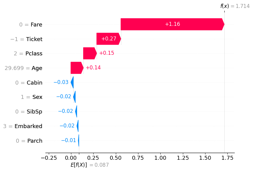
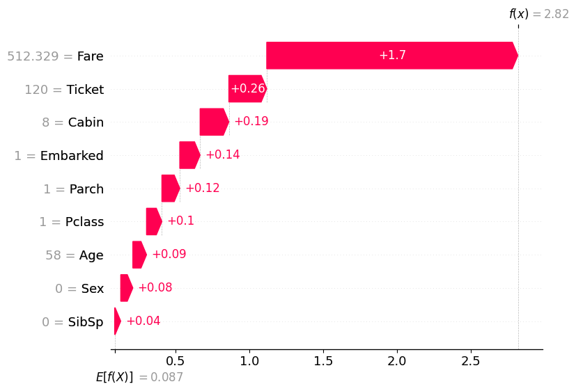
⚠️ Please note that the feature values shown on the charts below are transformed into an internal representation; they may be encoded or modified based on internal preprocessing. Refer to the original datasets for the actual feature values.

⚠️ The detector has seen this dataset; the may result in overly optimistic estimates. Although the anomaly score in the explanation might not match, the magnitude of the feature scores can still be utilized to evaluate the impact of the feature on the anomaly score.

Top-5 test_data anomalies (total: 7)

	Pclass	Name	Sex	Age	SibSp	Parch	Ticket	Fare	Cabin	Embarked	score
343	1	Cardeza, Mrs. James Warburton Martinez (Charlo...	female	58.000000	0	1	PC 17755	512.3292	B51 B53 B55	C	2.851073
263	3	Klasen, Miss. Gertrud Emilia	female	1.000000	1	1	350405	12.1833	NaN	S	1.963183
307	3	Aks, Master. Philip Frank	male	0.830000	0	1	392091	9.3500	NaN	S	1.827309
409	3	Peacock, Miss. Treasteall	female	3.000000	1	1	SOTON/O.Q. 3101315	13.7750	NaN	S	1.778720
266	1	Chisholm, Mr. Roderick Robert Crispin	male	29.699118	0	0	112051	0.0000	NaN	S	1.744582

⚠️ Please note that the feature values shown on the charts below are transformed into an internal representation; they may be encoded or modified based on internal preprocessing. Refer to the original datasets for the actual feature values.

Visualize Anomalies

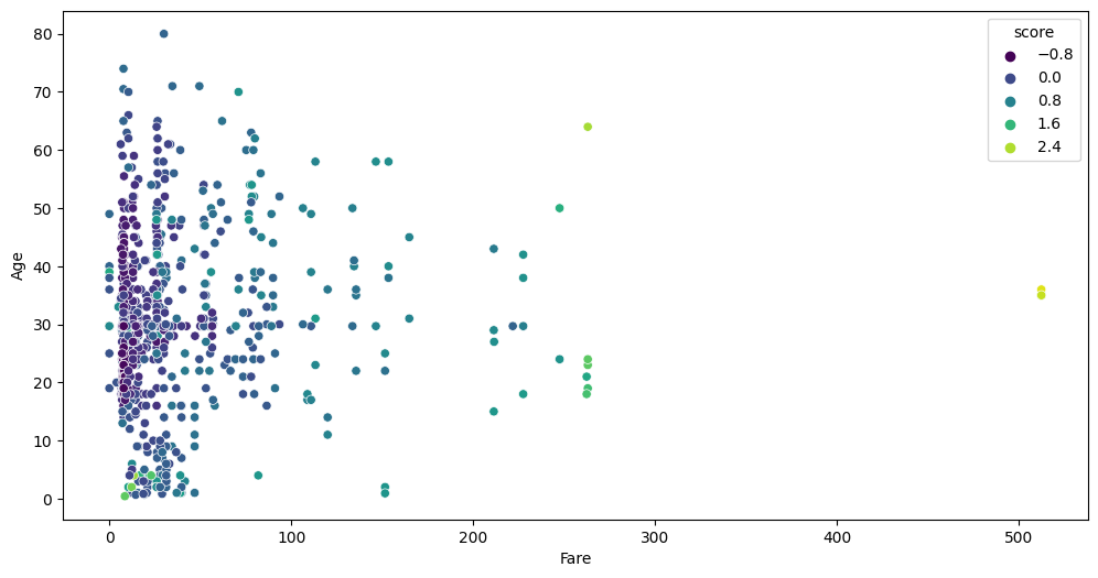
As we can see from the feature impact charts, the anomaly scores are primarily influenced by the Fare and Age features. Let’s take a look at a visual slice of the feature space. We can get the scores from state under anomaly_detection.scores.<dataset> keys:

train_anomaly_scores = state.anomaly_detection.scores.train_data
test_anomaly_scores = state.anomaly_detection.scores.test_data

auto.analyze_interaction(train_data=df_train.join(train_anomaly_scores), x="Fare", y="Age", hue="score", chart_args=dict(palette='viridis'))

auto.analyze_interaction(train_data=df_test.join(test_anomaly_scores), x="Fare", y="Age", hue="score", chart_args=dict(palette='viridis'))

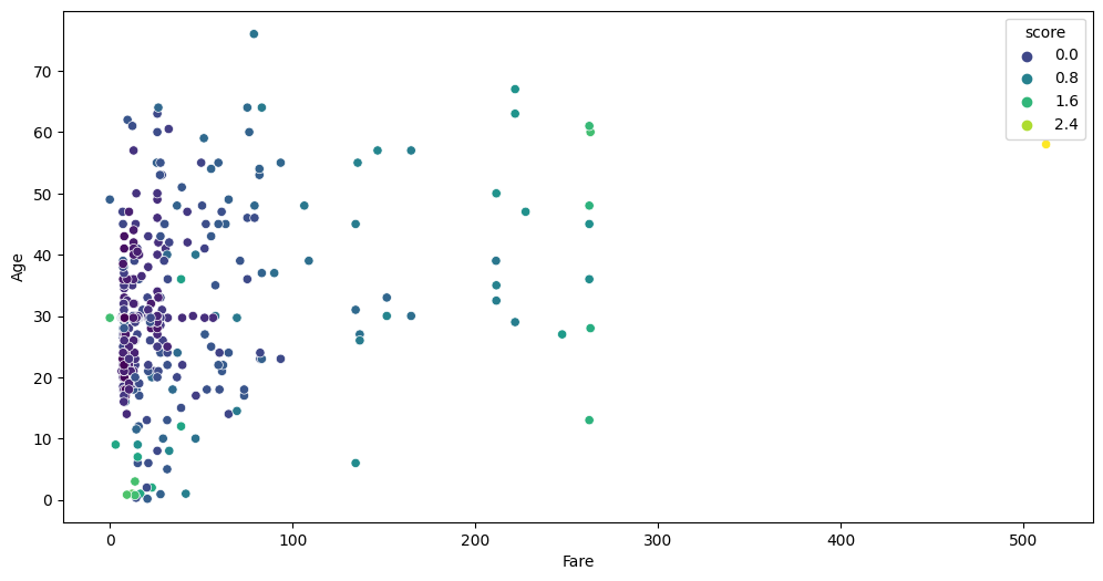
The data points in the lower left corner don’t appear to be anomalies. However, this is only because we are looking at a slice of the 11-dimensional data. While it might not seem like an anomaly in this slice, it is salient in other dimensions.

In conclusion, in this tutorial we’ve guided you through the process of using AutoGluon for anomaly detection. We’ve covered how to automatically detect anomalies with just a few lines of code. We also explored finding and visualizing the top detected anomalies, which can help you better understand and address the underlying issues. Lastly, we explored how to find the main contributing factors that led to a data point being marked as an anomaly, allowing you to pinpoint the root causes and take appropriate action.