Automated Quick Model Fit

The purpose of this feature is to provide a quick and easy way to obtain a preliminary understanding of the relationships between the target variable and the independent variables in a dataset.

This functionality automatically splits the training data, fits a simple regression or classification model to the data and generates insights: model performance metrics, feature importance and prediction result insights.

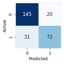
To inspect the prediction quality, a confusion matrix is displayed for classification problems and scatter plot for regression problems. Both representation allow the user to see the difference between actual and predicted values.

The insights highlight two subsets of the model predictions:

• Predictions with the largest classification error. Rows listed in this section are candidates for inspecting why the model made the mistakes

• Predictions with the least distance from the other class. Rows in this category are most ‘undecided’. They are useful as examples of data which is close to a decision boundary between the classes. The model would benefit from having more data for similar cases.

Classification Example

We will start with getting the titanic dataset and performing a quick one-line overview to get the information.

import pandas as pd
import autogluon.eda.auto as auto

df_train = pd.read_csv('https://autogluon.s3.amazonaws.com/datasets/titanic/train.csv')
df_test = pd.read_csv('https://autogluon.s3.amazonaws.com/datasets/titanic/test.csv')
target_col = 'Survived'

state = auto.quick_fit(
    df_train, 
    target_col, 
    return_state=True,
    show_feature_importance_barplots=True
)

No path specified. Models will be saved in: "AutogluonModels/ag-20230629_224529/"

Model Prediction for Survived

Using validation data for Test points

Model Leaderboard

	model	score_test	score_val	pred_time_test	pred_time_val	fit_time	pred_time_test_marginal	pred_time_val_marginal	fit_time_marginal	stack_level	can_infer	fit_order
0	LightGBMXT	0.809701	0.856	0.004057	0.003366	0.23442	0.004057	0.003366	0.23442	1	True	1

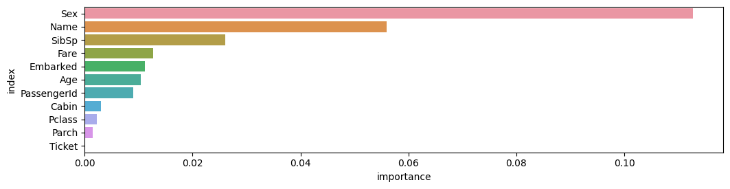
Feature Importance for Trained Model

	importance	stddev	p_value	n	p99_high	p99_low
Sex	0.112687	0.013033	0.000021	5	0.139522	0.085851
Name	0.055970	0.009140	0.000082	5	0.074789	0.037151
SibSp	0.026119	0.010554	0.002605	5	0.047850	0.004389
Fare	0.012687	0.009730	0.021720	5	0.032721	-0.007348
Embarked	0.011194	0.006981	0.011525	5	0.025567	-0.003179
Age	0.010448	0.003122	0.000853	5	0.016876	0.004020
PassengerId	0.008955	0.005659	0.012022	5	0.020607	-0.002696
Cabin	0.002985	0.006675	0.186950	5	0.016729	-0.010758
Pclass	0.002239	0.005659	0.213159	5	0.013890	-0.009413
Parch	0.001493	0.002044	0.088904	5	0.005701	-0.002716
Ticket	0.000000	0.000000	0.500000	5	0.000000	0.000000

Rows with the highest prediction error

Rows in this category worth inspecting for the causes of the error

	PassengerId	Pclass	Name	Sex	Age	SibSp	Parch	Ticket	Fare	Cabin	Embarked	Survived	0	1	error
498	499	1	Allison, Mrs. Hudson J C (Bessie Waldo Daniels)	female	25.0	1	2	113781	151.5500	C22 C26	S	0	0.046788	0.953212	0.906424
267	268	3	Persson, Mr. Ernst Ulrik	male	25.0	1	0	347083	7.7750	NaN	S	1	0.932024	0.067976	0.864047
569	570	3	Jonsson, Mr. Carl	male	32.0	0	0	350417	7.8542	NaN	S	1	0.922265	0.077735	0.844530
283	284	3	Dorking, Mr. Edward Arthur	male	19.0	0	0	A/5. 10482	8.0500	NaN	S	1	0.921180	0.078820	0.842361
821	822	3	Lulic, Mr. Nikola	male	27.0	0	0	315098	8.6625	NaN	S	1	0.919709	0.080291	0.839419
301	302	3	McCoy, Mr. Bernard	male	NaN	2	0	367226	23.2500	NaN	Q	1	0.918546	0.081454	0.837093
288	289	2	Hosono, Mr. Masabumi	male	42.0	0	0	237798	13.0000	NaN	S	1	0.907043	0.092957	0.814085
36	37	3	Mamee, Mr. Hanna	male	NaN	0	0	2677	7.2292	NaN	C	1	0.906803	0.093197	0.813605
127	128	3	Madsen, Mr. Fridtjof Arne	male	24.0	0	0	C 17369	7.1417	NaN	S	1	0.906605	0.093395	0.813210
391	392	3	Jansson, Mr. Carl Olof	male	21.0	0	0	350034	7.7958	NaN	S	1	0.905367	0.094633	0.810734

Rows with the least distance vs other class

Rows in this category are the closest to the decision boundary vs the other class and are good candidates for additional labeling

	PassengerId	Pclass	Name	Sex	Age	SibSp	Parch	Ticket	Fare	Cabin	Embarked	Survived	0	1	error
347	348	3	Davison, Mrs. Thomas Henry (Mary E Finck)	female	NaN	1	0	386525	16.1000	NaN	S	1	0.510786	0.489214	0.021572
192	193	3	Andersen-Jensen, Miss. Carla Christine Nielsine	female	19.0	1	0	350046	7.8542	NaN	S	1	0.512167	0.487833	0.024334
172	173	3	Johnson, Miss. Eleanor Ileen	female	1.0	1	1	347742	11.1333	NaN	S	1	0.526793	0.473207	0.053585
328	329	3	Goldsmith, Mrs. Frank John (Emily Alice Brown)	female	31.0	1	1	363291	20.5250	NaN	S	1	0.531574	0.468426	0.063149
593	594	3	Bourke, Miss. Mary	female	NaN	0	2	364848	7.7500	NaN	Q	0	0.463840	0.536160	0.072319
376	377	3	Landergren, Miss. Aurora Adelia	female	22.0	0	0	C 7077	7.2500	NaN	S	1	0.549471	0.450529	0.098942
607	608	1	Daniel, Mr. Robert Williams	male	27.0	0	0	113804	30.5000	NaN	S	1	0.558802	0.441198	0.117605
113	114	3	Jussila, Miss. Katriina	female	20.0	1	0	4136	9.8250	NaN	S	0	0.439738	0.560262	0.120524
889	890	1	Behr, Mr. Karl Howell	male	26.0	0	0	111369	30.0000	C148	C	1	0.568476	0.431524	0.136952
18	19	3	Vander Planke, Mrs. Julius (Emelia Maria Vande...	female	31.0	1	0	345763	18.0000	NaN	S	0	0.418177	0.581823	0.163645

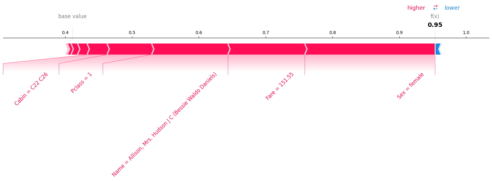
Explain rows

Let’s take a look what were the contibuting factors in the row with the highest error. auto.explain_rows can perform SHAP analysis for the specified rows and render it either using force or waterfall layout.

auto.explain_rows(
    train_data=df_train,
    model=state.model,
    display_rows=True,
    rows=state.model_evaluation.highest_error[:1]
)

	PassengerId	Pclass	Name	Sex	Age	SibSp	Parch	Ticket	Fare	Cabin	Embarked	Survived	0	1	error
498	499	1	Allison, Mrs. Hudson J C (Bessie Waldo Daniels)	female	25.0	1	2	113781	151.55	C22 C26	S	0	0.046788	0.953212	0.906424

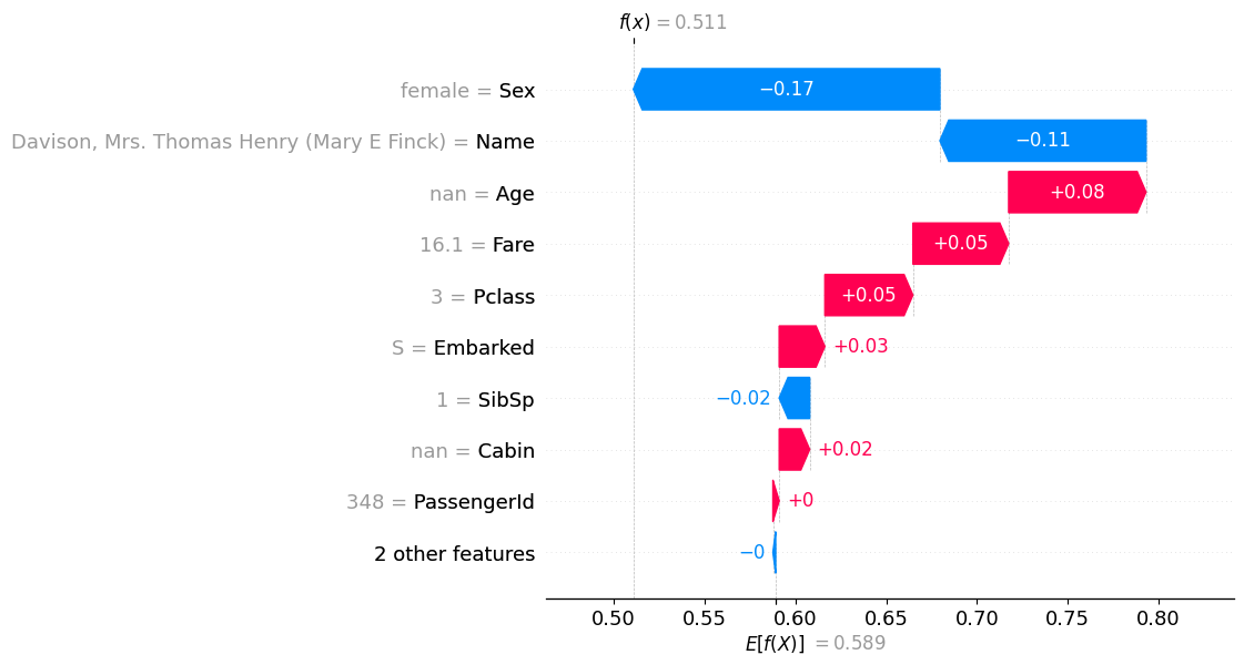
Next we are going to inspect the most undecided rows that were misclassified. This time we will use waterfall layout.

auto.explain_rows(
    train_data=df_train,
    model=state.model,
    display_rows=True,
    plot="waterfall",
    rows=state.model_evaluation.undecided[:1],
)

	PassengerId	Pclass	Name	Sex	Age	SibSp	Parch	Ticket	Fare	Cabin	Embarked	Survived	0	1	error
347	348	3	Davison, Mrs. Thomas Henry (Mary E Finck)	female	NaN	1	0	386525	16.1	NaN	S	1	0.510786	0.489214	0.021572

Regression Example

In the previous section we tried a classification example. Let’s try a regression. It has a few differences. We are also going to return the state to retrieve the fitted model and use it to predict test values later.

It is a large dataset, so we’ll keep only a few columns for this tutorial.

df_train = pd.read_csv('https://autogluon.s3.amazonaws.com/datasets/AmesHousingPriceRegression/train_data.csv')
df_test = pd.read_csv('https://autogluon.s3.amazonaws.com/datasets/AmesHousingPriceRegression/test_data.csv')
target_col = 'SalePrice'

keep_cols = [
  'Overall.Qual', 'Gr.Liv.Area', 'Neighborhood', 'Total.Bsmt.SF', 'BsmtFin.SF.1',
  'X1st.Flr.SF', 'Bsmt.Qual', 'Garage.Cars', 'Half.Bath', 'Year.Remod.Add', target_col
]

df_train = df_train[[c for c in df_train.columns if c in keep_cols]][:500]
df_test = df_test[[c for c in df_test.columns if c in keep_cols]][:500]


state = auto.quick_fit(df_train, target_col, fit_bagging_folds=3, return_state=True)

No path specified. Models will be saved in: "AutogluonModels/ag-20230629_224544/"

Model Prediction for SalePrice

Using validation data for Test points

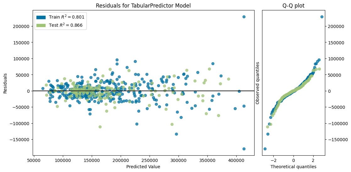
Model Leaderboard

	model	score_test	score_val	pred_time_test	pred_time_val	fit_time	pred_time_test_marginal	pred_time_val_marginal	fit_time_marginal	stack_level	can_infer	fit_order
0	LightGBMXT_BAG_L1	-26374.815144	-31051.161005	0.017108	0.009785	0.62157	0.017108	0.009785	0.62157	1	True	1

Feature Importance for Trained Model

	importance	stddev	p_value	n	p99_high	p99_low
Overall.Qual	15742.512622	1159.851290	0.000004	5	18130.662459	13354.362785
Gr.Liv.Area	11779.745065	1037.331690	0.000007	5	13915.625352	9643.864778
Year.Remod.Add	5634.405015	1378.973430	0.000398	5	8473.730367	2795.079663
X1st.Flr.SF	5561.463571	607.354702	0.000017	5	6812.015297	4310.911845
Total.Bsmt.SF	4273.958639	612.409034	0.000049	5	5534.917303	3012.999974
Garage.Cars	4195.617443	729.492238	0.000105	5	5697.652044	2693.582842
BsmtFin.SF.1	3436.181072	389.397237	0.000019	5	4237.955366	2634.406779
Half.Bath	2492.748327	802.313584	0.001128	5	4144.723085	840.773569
Bsmt.Qual	218.409613	185.023428	0.028804	5	599.375409	-162.556184
Neighborhood	71.437279	24.624389	0.001456	5	122.139236	20.735322

Rows with the highest prediction error

Rows in this category worth inspecting for the causes of the error

	Neighborhood	Overall.Qual	Year.Remod.Add	Bsmt.Qual	BsmtFin.SF.1	Total.Bsmt.SF	X1st.Flr.SF	Gr.Liv.Area	Half.Bath	Garage.Cars	SalePrice	SalePrice_pred	error
134	Edwards	6	1966	Gd	0.0	697.0	1575	2201	0	2.0	274970	164228.937500	110741.062500
90	Timber	10	2007	Ex	0.0	1824.0	1824	1824	0	3.0	392000	288768.218750	103231.781250
468	NridgHt	9	2003	Ex	1972.0	2452.0	2452	2452	0	3.0	445000	369170.468750	75829.531250
45	NridgHt	9	2006	Ex	0.0	1704.0	1722	2758	1	3.0	418000	347761.937500	70238.062500
322	NoRidge	8	1993	Gd	1129.0	1390.0	1402	2225	1	3.0	285000	353280.843750	68280.843750
26	Mitchel	5	2006	NaN	0.0	0.0	1771	1771	0	2.0	115000	181614.609375	66614.609375
233	NoRidge	8	2000	Gd	655.0	1145.0	1145	2198	1	3.0	250000	313840.656250	63840.656250
469	MeadowV	6	1973	Gd	837.0	942.0	1291	2521	1	2.0	151400	214016.359375	62616.359375
15	Crawfor	7	1992	TA	0.0	851.0	867	1718	1	2.0	238000	175619.453125	62380.546875
318	Crawfor	7	2002	Gd	1406.0	1902.0	1902	1902	0	2.0	335000	278283.031250	56716.968750

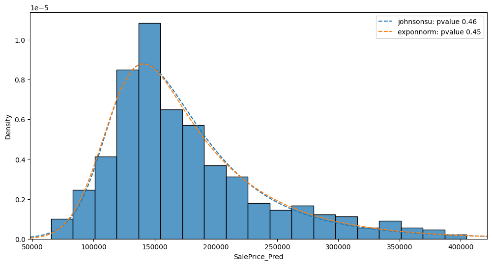
Using a fitted model

Now let’s get the model from state, perform the prediction on df_test and quickly visualize the results using auto.analyze_interaction() tool:

model = state.model
y_pred = model.predict(df_test)
auto.analyze_interaction(
    train_data=pd.DataFrame({'SalePrice_Pred': y_pred}), 
    x='SalePrice_Pred', 
    fit_distributions=['johnsonsu', 'norm', 'exponnorm']
)