Forecasting Time Series - Quick Start

Via a simple fit() call, AutoGluon can train and tune

• simple forecasting models (e.g., ARIMA, ETS, Theta),

• powerful deep learning models (e.g., DeepAR, Temporal Fusion Transformer),

• tree-based models (e.g., XGBoost, CatBoost, LightGBM),

• an ensemble that combines predictions of other models

to produce multi-step ahead probabilistic forecasts for univariate time series data.

This tutorial demonstrates how to quickly start using AutoGluon to generate hourly forecasts for the M4 forecasting competition. For a short summary of how to train models and make forecasts in a few lines of code with autogluon.timeseries, scroll to the bottom of this page. Also check out the AutoGluon-TimeSeries cheat sheet.

Loading time series data as a TimeSeriesDataFrame

First, we import some required modules

import pandas as pd
import matplotlib.pyplot as plt

from autogluon.timeseries import TimeSeriesDataFrame, TimeSeriesPredictor

To use autogluon.timeseries, we will only need the following two classes:

• TimeSeriesDataFrame stores a dataset consisting of multiple time series.

• TimeSeriesPredictor takes care of fitting, tuning and selecting the best forecasting models, as well as generating new forecasts.

We start by downloading the M4 Hourly dataset from the official website (click on the arrow to show the preprocessing code).

Loader for the M4 Hourly dataset

pd.set_option('display.max_rows', 6)  # Save space when printing

M4_INFO_URL = "https://github.com/Mcompetitions/M4-methods/raw/master/Dataset/M4-info.csv"
M4_HOURLY_URL = "https://github.com/Mcompetitions/M4-methods/raw/master/Dataset/Train/Hourly-train.csv"

def download_m4_hourly_dataset(save_path):
    metadata = pd.read_csv(M4_INFO_URL)
    metadata = metadata[metadata["SP"] == "Hourly"].set_index("M4id")
    data = pd.read_csv(M4_HOURLY_URL, index_col="V1")
    results = []
    for item_id in metadata.index:
        time_series = data.loc[item_id].dropna().values
        start_time = pd.Timestamp(metadata.loc[item_id]["StartingDate"])
        timestamps = pd.date_range(start_time, freq="H", periods=len(time_series))
        results.append(pd.DataFrame({"M4id": [item_id] * len(time_series), "Date": timestamps, "Value": time_series}))
    result = pd.concat(results, ignore_index=True)
    result.to_csv(save_path, index=False)

download_m4_hourly_dataset("m4_hourly.csv")

The M4 dataset contains time series from various domains like finance, demography and economics. Our goal is to forecast the future values of each time series in the dataset given the past observations.

We load the dataset as a pandas.DataFrame

df = pd.read_csv(
    "m4_hourly.csv",
    parse_dates=["Date"],  # make sure that pandas parses the dates
)
df

	M4id	Date	Value
0	H1	2015-01-07 12:00:00	605.0
1	H1	2015-01-07 13:00:00	586.0
2	H1	2015-01-07 14:00:00	586.0
...	...	...	...
353497	H414	2017-06-06 09:00:00	35.0
353498	H414	2017-06-06 10:00:00	26.0
353499	H414	2017-06-06 11:00:00	17.0

353500 rows × 3 columns

Each row of the data frame contains a single observation (timestep) of a single time series represented by

• unique ID of the time series ("M4id")

• timestamp of the observation ("Date") as a pandas.Timestamp

• numeric value of the time series ("Value")

The raw dataset should always follow this format with at least three columns for unique ID, timestamp, and target value, but the names of these columns can be arbitrary. It is important, however, that we provide the names of the columns when constructing a TimeSeriesDataFrame that is used by AutoGluon. AutoGluon will raise an exception if the data doesn’t match the expected format.

ts_dataframe = TimeSeriesDataFrame.from_data_frame(
    df,
    id_column="M4id",  # column that contains unique ID of each time series
    timestamp_column="Date",  # column that contains timestamps of each observation
)
ts_dataframe

		Value
item_id	timestamp
H1	2015-01-07 12:00:00	605.0
	2015-01-07 13:00:00	586.0
	2015-01-07 14:00:00	586.0
...	...	...
H414	2017-06-06 09:00:00	35.0
	2017-06-06 10:00:00	26.0
	2017-06-06 11:00:00	17.0

353500 rows × 1 columns

We refer to each individual time series stored in a TimeSeriesDataFrame as an item. For example, items might correspond to different products in demand forecasting, or to different stocks in financial datasets. This setting is also referred to as a panel of time series. Note that this is not the same as multivariate forecasting — AutoGluon generates forecasts for each time series individually, without modeling interactions between different items (time series).

TimeSeriesDataFrame inherits from pandas.DataFrame, so all attributes and methods of pandas.DataFrame are also available in a TimeSeriesDataFrame. Note how TimeSeriesDataFrame organizes the data with a pandas.MultiIndex: the first level of the index corresponds to the item ID and the second level contains the timestamp when each observation was made. For example, we can use the loc accessor to access each individual time series.

ts_dataframe.loc["H2"].head()

	Value
timestamp
2015-01-07 12:00:00	3124.0
2015-01-07 13:00:00	2990.0
2015-01-07 14:00:00	2862.0
2015-01-07 15:00:00	2809.0
2015-01-07 16:00:00	2544.0

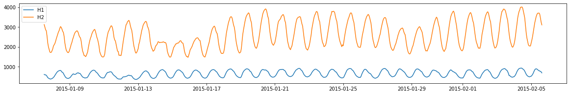
We can also plot some of the time series in the dataset

plt.figure(figsize=(20, 3))
for item_id in ["H1", "H2"]:
    plt.plot(ts_dataframe.loc[item_id], label=item_id)
plt.legend();

Forecasting problem formulation

Models in autogluon.timeseries provide probabilistic forecasts of time series multiple steps into the future. We choose the number of these steps—the prediction length (also known as the forecast horizon) depending on our task. For example, our dataset contains time series measured at hourly frequency, so we set prediction_length = 48 to train models that forecast 48 hours into the future. Moreover, forecasts are probabilistic: in addition to predicting the mean (expected value) of the time series in the future, models also provide the quantiles of the forecast distribution.

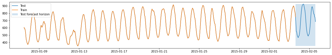
In order to report realistic results for how AutoGluon will perform on unseen data; we will split our dataset into a training set, used to train & tune models, and a test set used to evaluate the final performance. In forecasting, this is usually done by hiding the last prediction_length steps of each time series during training, and only using these last steps to evaluate the forecast quality (also known as “out of time validation”). We perform this split using the slice_by_timestep method of TimeSeriesDataFrame.

prediction_length = 48

test_data = ts_dataframe  # the full data set

# last prediction_length timesteps of each time series are excluded, akin to `x[:-48]`
train_data = ts_dataframe.slice_by_timestep(None, -prediction_length)

Below, we plot the training and test parts of the time series for a single country, and mark the test forecast horizon. We will compute the test scores by measuring how well the forecast generated by a model matches the actually observed values in the forecast horizon.

Training time series models with TimeSeriesPredictor.fit

Below we instantiate a TimeSeriesPredictor object and instruct AutoGluon to fit models that can forecast up to 48 timesteps into the future (prediction_length) and save them in the folder ./autogluon-m4-hourly. We also specify that AutoGluon should rank models according to mean absolute percentage error (MAPE), and that data that we want to forecast is stored in the column "Value" of the TimeSeriesDataFrame.

predictor = TimeSeriesPredictor(
    path="autogluon-m4-hourly",
    target="Value",
    prediction_length=prediction_length,
    eval_metric="MAPE",
)

predictor.fit(
    train_data,
    presets="medium_quality",
    time_limit=600,
)

================ TimeSeriesPredictor ================
TimeSeriesPredictor.fit() called
Setting presets to: medium_quality
Fitting with arguments:
{'enable_ensemble': True,
 'evaluation_metric': 'MAPE',
 'hyperparameter_tune_kwargs': None,
 'hyperparameters': 'medium_quality',
 'prediction_length': 48,
 'random_seed': None,
 'target': 'Value',
 'time_limit': 600}
Provided training data set with 333628 rows, 414 items (item = single time series). Average time series length is 805.9.
Training artifacts will be saved to: /home/ci/autogluon/docs/_build/eval/tutorials/timeseries/autogluon-m4-hourly
=====================================================
AutoGluon will save models to autogluon-m4-hourly/
AutoGluon will gauge predictive performance using evaluation metric: 'MAPE'
    This metric's sign has been flipped to adhere to being 'higher is better'. The reported score can be multiplied by -1 to get the metric value.
tuning_data is None. Will use the last prediction_length = 48 time steps of each time series as a hold-out validation set.

Starting training. Start time is 2022-12-13 01:40:59
Models that will be trained: ['Naive', 'SeasonalNaive', 'ETS', 'Theta', 'ARIMA', 'AutoGluonTabular', 'DeepAR']
Training timeseries model Naive. Training for up to 599.87s of the 599.87s of remaining time.
    -0.3718       = Validation score (-MAPE)
    0.00    s     = Training runtime
    6.30    s     = Validation (prediction) runtime
Training timeseries model SeasonalNaive. Training for up to 593.55s of the 593.55s of remaining time.
    -0.1922       = Validation score (-MAPE)
    0.00    s     = Training runtime
    1.16    s     = Validation (prediction) runtime
Training timeseries model ETS. Training for up to 592.37s of the 592.37s of remaining time.
    -0.3554       = Validation score (-MAPE)
    0.00    s     = Training runtime
    109.21  s     = Validation (prediction) runtime
Training timeseries model Theta. Training for up to 483.14s of the 483.14s of remaining time.
    -0.2136       = Validation score (-MAPE)
    0.00    s     = Training runtime
    35.81   s     = Validation (prediction) runtime
Training timeseries model ARIMA. Training for up to 447.30s of the 447.30s of remaining time.
    -0.5144       = Validation score (-MAPE)
    0.00    s     = Training runtime
    44.41   s     = Validation (prediction) runtime
Training timeseries model AutoGluonTabular. Training for up to 402.87s of the 402.87s of remaining time.
    -0.0973       = Validation score (-MAPE)
    70.98   s     = Training runtime
    3.71    s     = Validation (prediction) runtime
Training timeseries model DeepAR. Training for up to 328.18s of the 328.18s of remaining time.
    -0.1266       = Validation score (-MAPE)
    149.85  s     = Training runtime
    4.00    s     = Validation (prediction) runtime
Fitting simple weighted ensemble.
    -0.0973       = Validation score (-MAPE)
    162.88  s     = Training runtime
    7.71    s     = Validation (prediction) runtime
Training complete. Models trained: ['Naive', 'SeasonalNaive', 'ETS', 'Theta', 'ARIMA', 'AutoGluonTabular', 'DeepAR', 'WeightedEnsemble']
Total runtime: 630.95 s
Best model: WeightedEnsemble
Best model score: -0.0973

<autogluon.timeseries.predictor.TimeSeriesPredictor at 0x7f04ccbb2b80>

Here we used the "medium_quality" presets and limited the training time to 10 minutes (600 seconds). The presets define which models AutoGluon will try to fit. For medium_quality presets, these are simple baselines (Naive, SeasonalNaive), statistical models (ARIMA, ETS, Theta), tree-based models XGBoost, LightGBM and CatBoost wrapped by AutoGluonTabular, a deep learning model DeepAR, and a weighted ensemble combining these. Other available presets for TimeSeriesPredictor are "fast_training" "high_quality" and "best_quality". Higher quality presets will usually produce more accurate forecasts but take longer to train and may produce less computationally efficient models.

Inside fit(), AutoGluon will train as many models as possible within the given time limit. Trained models are then ranked based on their performance on an internal validation set. By default, this validation set is constructed by holding out the last prediction_length timesteps of each time series in train_data.

Evaluating the performance of different models

We can view the test performance of each model AutoGluon has trained via the leaderboard() method. We provide the test data set to the leaderboard function to see how well our fitted models are doing on the held out test data. The leaderboard also includes the validation scores computed on the internal validation dataset.

In AutoGluon leaderboards, higher scores always correspond to better predictive performance. Therefore our MAPE scores are multiplied by -1, such that higher “negative MAPE”s correspond to more accurate forecasts.

predictor.leaderboard(test_data, silent=True)

Additional data provided, testing on additional data. Resulting leaderboard will be sorted according to test score (score_test).

	model	score_test	score_val	pred_time_test	pred_time_val	fit_time_marginal	fit_order
0	AutoGluonTabular	-0.134804	-0.097343	3.715563	3.710325	70.975730	6
1	WeightedEnsemble	-0.134815	-0.097259	40.152865	7.714724	162.878917	8
2	DeepAR	-0.164160	-0.126642	36.907747	4.004399	149.852732	7
...	...	...	...	...	...	...	...
5	Naive	-0.376335	-0.371842	6.144834	6.296322	0.003169	1
6	ETS	-0.514677	-0.355394	108.055015	109.208286	0.001525	3
7	ARIMA	-0.570275	-0.514399	44.066189	44.408719	0.001580	5

8 rows × 7 columns

Generating forecasts with TimeSeriesPredictor.predict

We can now use the fitted TimeSeriesPredictor to make predictions. By default, AutoGluon will make forecasts using the model that had the best validation score (as shown in the leaderboard). Let’s use the predictor to generate forecasts starting from the end of the time series in train_data

predictions = predictor.predict(train_data)
predictions.head()

Model not specified in predict, will default to the model with the best validation score: WeightedEnsemble

		mean	0.1	0.2	0.3	0.4	0.5	0.6	0.7	0.8	0.9
item_id	timestamp
H1	2015-02-03 16:00:00	661.771644	528.747822	574.402724	607.305205	635.445695	661.660249	687.965532	716.088843	749.015370	794.966803
	2015-02-03 17:00:00	564.427770	431.633816	477.180554	510.050814	538.126973	564.361066	590.658266	618.746708	651.610390	697.302567
	2015-02-03 18:00:00	522.741473	389.753903	435.459457	468.384505	496.528754	522.803124	549.038642	577.120841	610.014356	655.623966
	2015-02-03 19:00:00	480.616592	347.653460	393.315141	426.285392	454.363555	480.589916	506.851500	534.982443	567.899552	613.584161
	2015-02-03 20:00:00	459.024806	326.039030	371.688073	404.601741	432.746835	458.994874	485.323435	513.462600	546.334049	591.879379

Predictions are also stored as a TimeSeriesDataFrame. However, now the columns contain the mean and quantile predictions of each model. The quantile forecasts give us an idea about the range of possible outcomes. For example, if the "0.1" quantile is equal to 501.3, it means that the model predicts a 10% chance that the target value will be below 501.3.

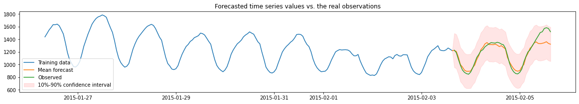
We will now visualize the forecast and the actually observed values for one of the time series in the dataset. We plot the mean forecast, as well as the 10% and 90% quantiles to show the range of potential outcomes.

plt.figure(figsize=(20, 3))

item_id = "H3"
y_past = train_data.loc[item_id]["Value"]
y_pred = predictions.loc[item_id]
y_true = test_data.loc[item_id]["Value"][-prediction_length:]

# prepend the last value of true range to predicted range for plotting continuity
y_pred.loc[y_past.index[-1]] = [y_past[-1]] * 10
y_pred = y_pred.sort_index()

plt.plot(y_past[-200:], label="Training data")
plt.plot(y_pred["mean"], label="Mean forecast")
plt.plot(y_true, label="Observed")

plt.fill_between(
    y_pred.index, y_pred["0.1"], y_pred["0.9"], color="red", alpha=0.1, label=f"10%-90% confidence interval"
)
plt.title("Forecasted time series values vs. the real observations")
plt.legend();

Summary

We used autogluon.timeseries to make probabilistic multi-step forecasts on the M4 Hourly dataset. Here is a short summary of the main steps for applying AutoGluon to make forecasts for the entire dataset using a few lines of code.

import pandas as pd

from autogluon.timeseries import TimeSeriesPredictor, TimeSeriesDataFrame

# Load the data into a TimeSeriesDataFrame
df = pd.read_csv(
    "m4_hourly.csv",
    parse_dates=["Date"],
)
ts_dataframe = TimeSeriesDataFrame.from_data_frame(
    df,
    id_column="M4id",  # name of the column with unique ID of each time series
    timestamp_column="Date",  # name of the column with timestamps of observations
)

# Create & fit the predictor
predictor = TimeSeriesPredictor(
    path="autogluon-m4-hourly",  # models will be saved in this folder
    target="Value",  # name of the column with time series values
    prediction_length=48,  # number of steps into the future to predict
    eval_metric="MAPE",  # other options: "MASE", "sMAPE", "mean_wQuantileLoss", "MSE", "RMSE"
).fit(
    train_data=ts_dataframe,
    presets="medium_quality",  # other options: "fast_training", "high_quality", "best_quality"
    time_limit=600,  # training time in seconds
)

# Generate the forecasts
predictions = predictor.predict(ts_dataframe)

Check out Forecasting Time Series - In Depth to learn about the advanced capabilities of AutoGluon for time series forecasting.