
Forecasting Time Series - Quick Start
Via a simple fit() call, AutoGluon can train
simple forecasting models (e.g., ARIMA, ETS),
powerful neural network-based models (e.g., DeepAR, Transformer, MQ-CNN),
and fit greedy weighted ensembles built on these
to produce multi-step ahead probabilistic forecasts for univariate time series data.
NOTE
autogluon.timeseries depends on Apache MXNet. Please install MXNet
by
python -m pip install mxnet>=1.9
or, if you are using a GPU with a matching MXNet package for your CUDA driver. See the MXNet documentation for more info.
This tutorial demonstrates how to quickly start using AutoGluon to produce forecasts of COVID-19 cases in a country given historical data from each country.
autogluon.timeseries provides the TimeSeriesPredictor and
TimeSeriesDataFrame classes for interacting with time series models.
TimeSeriesDataFrame contains time series data. The
TimeSeriesPredictor class provides the interface for fitting, tuning
and selecting forecasting models.
import pandas as pd
from matplotlib import pyplot as plt

from autogluon.timeseries import TimeSeriesPredictor, TimeSeriesDataFrame
TimeSeriesDataFrame objects hold time series data, often with
multiple “items” (time series) such as different products in demand
forecasting. This setting is also sometimes referred to as a “panel” of
time series. TimeSeriesDataFrame inherits from Pandas
DataFrame,
and the attributes and methods of pandas.DataFrames are available
in TimeSeriesDataFrames.
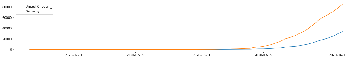
In our example, we work with COVID case data as of April 2020 where our
goal is to forecast the number of confirmed COVID cases for each country
in the data set. Below, we load time series data from an AWS S3
bucket, and prepare it for use in
autogluon.timeseries. Note that we make sure the date field is
parsed by pandas, and provide the columns containing the item
(id_column) and timestamps (timestamp_column) to
TimeSeriesDataFrame. We also plot the trajectories of COVID cases
with two example countries: Germany and the UK.
df = pd.read_csv(
    "https://autogluon.s3-us-west-2.amazonaws.com/datasets/CovidTimeSeries/train.csv",
    parse_dates=["Date"],
)

train_data = TimeSeriesDataFrame.from_data_frame(
    df,
    id_column="name",
    timestamp_column="Date",
)

plt.figure(figsize=(20, 3))
for country in ["United Kingdom_", "Germany_"]:
    plt.plot(train_data.loc[country], label=country)
plt.legend()
<matplotlib.legend.Legend at 0x7f5e90c7c1c0>
Note how TimeSeriesDataFrame objects organize the data with a
pandas.MultiIndex where the first level of the index corresponds
to the item (here, country) and the second level contains the dates for
which the values were observed. We can also use the loc accessor, as
in pandas, to access individual country data.
train_data.head()
| ConfirmedCases | ||
|---|---|---|
| item_id | timestamp | |
| Afghanistan_ | 2020-01-22 | 0.0 |
| 2020-01-23 | 0.0 | |
| 2020-01-24 | 0.0 | |
| 2020-01-25 | 0.0 | |
| 2020-01-26 | 0.0 |
train_data.loc['Afghanistan_'].head()
| ConfirmedCases | |
|---|---|
| timestamp | |
| 2020-01-22 | 0.0 |
| 2020-01-23 | 0.0 |
| 2020-01-24 | 0.0 |
| 2020-01-25 | 0.0 |
| 2020-01-26 | 0.0 |
The primary use case of autogluon.timeseries is time series
forecasting. In our example, our goal is to train models on COVID case
data that can forecast the future trajectory of cases given the past,
for each country in the data set. By default, autogluon.timeseries
supports multi-step ahead probabilistic forecasting. That is, multiple
time steps in the future can be forecasted, given that models are
trained with the prerequisite number of steps (also known as the
forecast horizon). Moreover, when trained models are used to predict
the future, the library will provide both "mean" forecasts–expected
values of the time series in the future, as well as quantiles of the
forecast distribution.
In order to train our forecasting models, we first split the data into
training and test data sets. In forecasting, this is often done via
excluding the last prediction_length many steps of the data set
during training, and only use these steps to compute validation scores
(also known as an “out of time” validation sample). We carry out this
split via the slice_by_timestep method provided by
TimeSeriesDataFrame which takes python slice objects.
prediction_length = 5

test_data = train_data.copy()  # the full data set

# the data set with the last prediction_length time steps included, i.e., akin to `a[:-5]`
train_data = train_data.slice_by_timestep(slice(None, -prediction_length))
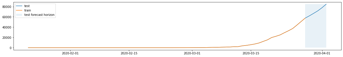
Below, for a single country we plot the training and test data sets showing how they overlap and explicitly mark the forecast horizon of the test data set. The test scores will be computed on forecasts provided for this range.
plt.figure(figsize=(20, 3))
plt.plot(test_data.loc["Germany_"], label="test")
plt.plot(train_data.loc["Germany_"], label="train")

test_range = (
    test_data.loc["Germany_"].index.max(),
    train_data.loc["Germany_"].index.max(),
)

plt.fill_betweenx(
    y=(0, test_data.loc["Germany_"]["ConfirmedCases"].max()),
    x1=test_range[0],
    x2=test_range[1],
    alpha=0.1,
    label="test forecast horizon",
)

plt.legend()
<matplotlib.legend.Legend at 0x7f5e90b3de80>
Below we instantiate a TimeSeriesPredictor object and instruct
AutoGluon to fit models that can forecast up to 5 time-points into the
future (prediction_length) and save them in the folder
./autogluon-covidforecast. We also specify that AutoGluon should
rank models according to mean absolute percentage error (MAPE) and that
the target field to be forecasted is "ConfirmedCases".
predictor = TimeSeriesPredictor(
    path="autogluon-covidforecast",
    target="ConfirmedCases",
    prediction_length=prediction_length,
    eval_metric="MAPE",
)
predictor.fit(
    train_data=train_data,
    presets="low_quality",
)
presets is set to low_quality
================ TimeSeriesPredictor ================
TimeSeriesPredictor.fit() called
Setting presets to: low_quality
Fitting with arguments:
{'evaluation_metric': 'MAPE',
 'hyperparameter_tune_kwargs': None,
 'hyperparameters': 'toy',
 'prediction_length': 5,
 'target_column': 'ConfirmedCases',
 'time_limit': None}
Provided training data set with 20971 rows, 313 items. Average time series length is 67.0.
Training artifacts will be saved to: /var/lib/jenkins/workspace/workspace/autogluon-timeseries-py3-v3/docs/_build/eval/tutorials/timeseries/autogluon-covidforecast
=====================================================
Validation data is None, will hold the last prediction_length 5 time steps out to use as validation set.

Starting training. Start time is 2022-07-18 23:49:39
Models that will be trained: ['AutoETS', 'SimpleFeedForward', 'DeepAR', 'ARIMA', 'Transformer']
Training timeseries model AutoETS.
    -0.3287       = Validation score (-MAPE)
    4.11    s     = Training runtime
    19.81   s     = Validation (prediction) runtime
Training timeseries model SimpleFeedForward.
    -0.3725       = Validation score (-MAPE)
    11.21   s     = Training runtime
    1.44    s     = Validation (prediction) runtime
Training timeseries model DeepAR.
    -0.7700       = Validation score (-MAPE)
    11.40   s     = Training runtime
    2.01    s     = Validation (prediction) runtime
Training timeseries model ARIMA.
    -0.3665       = Validation score (-MAPE)
    10.55   s     = Training runtime
    33.72   s     = Validation (prediction) runtime
Training timeseries model Transformer.
    -1.8190       = Validation score (-MAPE)
    8.65    s     = Training runtime
    1.90    s     = Validation (prediction) runtime
Fitting simple weighted ensemble.
    -0.3076       = Validation score (-MAPE)
    117.68  s     = Training runtime
    21.25   s     = Validation (prediction) runtime
Training complete. Models trained: ['AutoETS', 'SimpleFeedForward', 'DeepAR', 'ARIMA', 'Transformer', 'WeightedEnsemble']
Total runtime: 281.78 s
Best model: WeightedEnsemble
Best model score: -0.3076
<autogluon.timeseries.predictor.TimeSeriesPredictor at 0x7f5e900d46a0>
In a short amount of time AutoGluon fits four time series forecasting models on the training data. These models are three neural network forecasters: DeepAR, MQCNN, a simple feedforward neural network; and a simple exponential smoothing model with automatic parameter tuning: Auto-ETS. AutoGluon also constructs a weighted ensemble of these models capable of quantile forecasting.
We can view the test performance of each model AutoGluon has trained via
the leaderboard() method. We provide the test data set to the
leaderboard function to see how well our fitted models are doing on the
held out time frame. In AutoGluon leaderboards, higher scores always
correspond to better predictive performance. Therefore our MAPE scores
are presented with a “flipped” sign, such that higher “negative MAPE”s
correspond to better models.
predictor.leaderboard(test_data, silent=True)
Additional data provided, testing on additional data. Resulting leaderboard will be sorted according to test score (score_test).
Different set of items than those provided during training were provided for prediction. The model AutoETS will be re-trained on newly provided data
Different set of items than those provided during training were provided for prediction. The model ARIMA will be re-trained on newly provided data
Different set of items than those provided during training were provided for prediction. The model AutoETS will be re-trained on newly provided data
| model | score_test | score_val | pred_time_test | pred_time_val | fit_time_marginal | fit_order | |
|---|---|---|---|---|---|---|---|
| 0 | SimpleFeedForward | -0.188259 | -0.372513 | 1.509150 | 1.438922 | 11.205414 | 2 |
| 1 | WeightedEnsemble | -0.189813 | -0.307592 | 25.705786 | 21.253829 | 117.679210 | 6 |
| 2 | DeepAR | -0.240209 | -0.769969 | 1.935482 | 2.012790 | 11.402265 | 3 |
| 3 | AutoETS | -0.247532 | -0.328701 | 24.641734 | 19.814908 | 4.110266 | 1 |
| 4 | ARIMA | -0.286547 | -0.366499 | 45.391605 | 33.715822 | 10.547525 | 4 |
| 5 | Transformer | -0.297987 | -1.818996 | 2.011078 | 1.902087 | 8.653442 | 5 |
We can now use the TimeSeriesPredictor to look at actual forecasts.
By default, AutoGluon will select the best performing model to forecast
time series with. Let’s use the predictor to compute forecasts, and plot
forecasts for an example country.
predictions = predictor.predict(train_data)
Model not specified in predict, will default to the model with the best validation score: WeightedEnsemble
Different set of items than those provided during training were provided for prediction. The model AutoETS will be re-trained on newly provided data
plt.figure(figsize=(20, 3))

ytrue = train_data.loc['France_']["ConfirmedCases"]
ypred = predictions.loc['France_']

# prepend the last value of true range to predicted range for plotting continuity
ypred.loc[ytrue.index[-1]] = [ytrue[-1]] * 10
ypred = ypred.sort_index()

ytrue_test = test_data.loc['France_']["ConfirmedCases"][-5:]

plt.plot(ytrue[-30:], label="Training Data")
plt.plot(ypred["mean"], label="Mean Forecasts")
plt.plot(ytrue_test, label="Actual")

plt.fill_between(
    ypred.index, ypred["0.1"], ypred["0.9"], color="red", alpha=0.1
)
plt.title("COVID Case Forecasts in France, compared to actual trajectory")
_ = plt.legend()
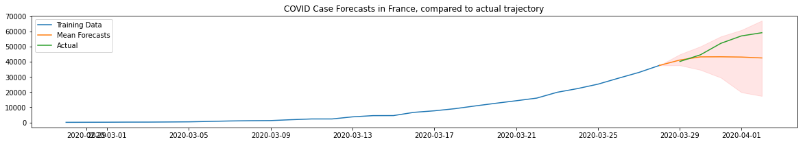
As we used a “toy” presets setting (presets="low_quality") our
forecasts may appear to not be doing very well. In realistic scenarios,
users can set presets to be one of: "best_quality",
"high_quality", "good_quality", "medium_quality". Higher
quality presets will generally produce superior forecasting accuracy but
take longer to train and may produce less efficient models.